Multiple Imputation by Chained Equations in SPSS
Discover Multiple Imputation by Chained Equations in SPSS! Learn how to perform, understand SPSS output, and report results in APA style. Check out this simple, easy-to-follow guide below for a quick read!
Struggling with MICE in SPSS! We’re here to help. We provide comprehensive support to academics and PhD students, encompassing assignments, dissertations, research, and additional services. Request Quote Now!

1. Introduction
Missing data is a common issue in research and can significantly affect the accuracy and validity of statistical analysis. One of the most robust approaches to address this problem is Multiple Imputation by Chained Equations (MICE). In this guide, we explain how MICE works and how to perform it effectively using SPSS.
2. What is Missing Data?
Missing data refers to the absence of information for one or more variables in a dataset. It can occur randomly or follow patterns, and it can be classified into three categories:
MCAR (Missing Completely at Random): The probability of missingness is unrelated to any observed or unobserved data.
MAR (Missing at Random): Missingness depends on other observed variables.
MNAR (Missing Not at Random): Missingness depends on the value itself or unobserved data.
Understanding the type of missingness is crucial for selecting an appropriate imputation strategy.
3. What is Multiple Imputation by Chained Equations?
MICE is an advanced method of multiple imputation that handles missing data by specifying a separate model for each variable with missing values. It iteratively fills in missing data by cycling through the variables, using observed and imputed data from other variables to predict missing values. This flexible method supports both continuous and categorical data and is particularly useful when variables have different distributions.
I. How The MICE Algorithm Mechanism Works
The MICE process involves the following steps:
1. Step: Initialize missing values with simple estimates (e.g., mean or median).
2. Step: Choose one variable with missing values. Use the other variables as predictors in a regression model.
3. Step: Impute missing values for the target variable using predicted values from the model.
4. Step: Repeat the process for the next variable with missing data.
5. Step: Cycle through all variables multiple times (iterations) to stabilize the estimates.
This chained approach continues until convergence is reached, and multiple complete datasets are generated.
II. How to Handle Missing Values with MICE
To handle missing values using MICE, you need to decide the imputation model for each variable type:
Linear regression for continuous variables
Logistic regression for binary variables
Multinomial logistic regression for categorical variables with more than two levels
Predictive mean matching (PMM) for more robust continuous imputation
MICE uses these models in an iterative fashion to create multiple plausible datasets that reflect uncertainty due to missingness.
III. When are MICE used for?
MICE is best used when:
The missing data mechanism is either Missing at Random (MAR) or Missing Completely at Random (MCAR).
You have a moderate-to-large sample size.
The dataset includes both categorical and continuous variables.
You want to conduct robust sensitivity analyses across multiple imputed datasets.
You aim to improve the validity and generalizability of your statistical inferences.
4. What is Multiple Data Imputation?
Multiple Imputation (MI) is a technique that:
Replaces missing values multiple times to create multiple complete datasets.
Analyzes each dataset separately.
Combines estimates using Rubin’s rules for valid inference.
MI helps capture the uncertainty associated with missing data and produces more accurate standard errors and confidence intervals than single imputation.
I. Rubin’s Rule for Multiple Imputation
Rubin’s Rule is a statistical method used to combine results from multiple imputed datasets. After missing data are filled in using multiple imputation, each dataset is analyzed separately. Rubin’s Rule then pools these results to produce a single, valid estimate that accounts for both:
Within-imputation variance (variability inside each dataset), and
Between-imputation variance (variability across the imputed datasets).
This rule ensures that standard errors, confidence intervals, and p-values properly reflect the uncertainty caused by missing data. SPSS automatically applies Rubin’s Rule when pooling estimates, allowing researchers to draw statistically sound inferences from multiply imputed data.
5. What are the Methods for Multiple Imputation in SPSS?
SPSS supports several MI methods, including:
Linear Regression (LR): Assumes normally distributed residuals; sensitive to outliers.
Predictive Mean Matching (PMM): A more robust alternative that uses observed values from similar cases rather than model predictions.
Both methods are accessible via Analyze → Multiple Imputation → Impute Missing Data Values, and can be specified under the Method section of the imputation model.
6. Comparing: Predictive Mean Matching vs Linear Regression
| Feature | Linear Regression (LR) | Predictive Mean Matching (PMM) |
|---|---|---|
| Assumes normal distribution | Yes | No |
| Handles outliers well | Poorly | Robust |
| Output values | Can be outside observed range | Limited to observed values |
| Suitable for skewed data | Less suitable | More suitable |
| Interpretation | Parametric | Semi-parametric |
PMM is often preferred when the variable to be imputed has a non-normal distribution or when preserving original scale and plausibility of values is important.
7. Why Should I Set an Iteration?
Iterations allow the model to stabilize the imputation process by cycling through variables multiple times. Each round refines the estimates based on updated imputations of other variables.
Typical setting: 10 iterations per imputed dataset.
More iterations may be needed for complex datasets with high missingness or multicollinearity.
SPSS allows users to set the number of iterations under the Number of Iterations tab during imputation setup.
8. Why Handling Missing Values Is Important in Statistical Analysis?
Failing to address missing data properly can lead to:
Biased estimates: If missingness is not random, ignoring it can distort your results.
Reduced statistical power: Loss of data means less information, resulting in wider confidence intervals and weaker significance.
Invalid assumptions: Many statistical models assume complete data. Violating this can compromise model validity.
By handling missing data thoughtfully—starting with an appropriate imputation strategy—you can ensure more reliable and interpretable results.
9. An Example for MICE using Predictive Mean Matching Methods
Suppose we are analyzing a dataset of 300 participants with variables Age, Income, and Education. The Income variable has 15% missing data, and is right-skewed.
Using PMM allows us to impute realistic income values based on matched cases with similar predicted values, avoiding unrealistic outliers that a regression model might produce.
This example demonstrates multiple imputation using PMM. To see an example using MICE with linear regression imputation, please visit the following page.
10. How to Perform Multiple Imputation in SPSS


Step by Step: Running Predictive Mean Matching in SPSS Statistics
To apply Predictive Mean Matching (PMM) in SPSS:
Go to
Analyze → Multiple Imputation → Impute Missing Data Values.Variables Tab:
Add variables with missing values to the Impute box.
Add predictors to the Predictors box.
Set a name for the imputed datasets (e.g.,
imp_).
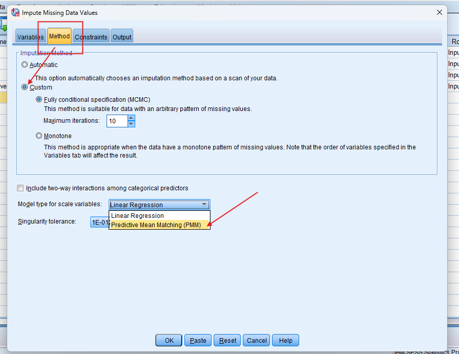
Method Tab:
Choose Fully Conditional Specification (FCS).
For each scale variable, select PMM as the imputation method.
Constraints Tab:
Set roles as needed: Impute only, Use as predictor, or Impute and use as predictor.
Output Tab:
Tick both options to display summaries and iteration history.
Set the number of imputations (e.g., 5) and iterations (e.g., 10), then click OK.
SPSS will create the imputed datasets, which can be viewed and analyzed using pooled results.
11. SPSS Output for Multiple Imputation using PMM


12. How to Interpret SPSS Output for MICE using Predictive Mean Matching
Once the imputation is complete, SPSS provides several key outputs:
Imputation Summary Table: Shows which variables were imputed, how many values were missing, and the method used (e.g., PMM).
Iteration History Table: Displays changes in variable means over the 10 iterations, confirming convergence.
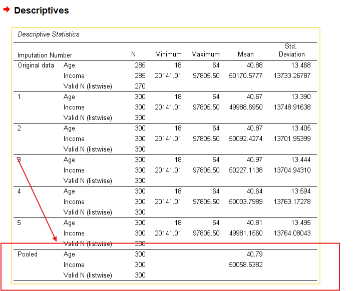
Descriptive Statistics Table: Reports the mean and standard deviation for each imputed variable across the datasets.
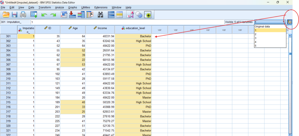
Imputed Dataset Viewer: You can review each imputed dataset individually via the drop-down in the SPSS Data Editor.
Pooled Results via Descriptives: After imputation, use
Analyze → Descriptive Statistics → Descriptives, check the “Pool results across imputations” box to obtain pooled means, standard deviations, or frequencies.
This allows the user to evaluate the plausibility and stability of the imputations, and confirms consistency across imputed datasets.
13. How to Report MICE with PMM Results
When reporting Predictive Mean Matching, include:
The software and method used (e.g., PMM under FCS in SPSS).
The number of imputations and iterations performed.
Key assumptions (e.g., data assumed to be MAR).
Pooled descriptive statistics (e.g., mean, SD).
The rationale for using PMM over alternatives.
Clarify that results were pooled using Rubin’s rules.
Get Help For Your SPSS Analysis
Embark on a seamless research journey with SPSSAnalysis.com, where our dedicated team provides expert data analysis assistance for students, academicians, and individuals. We ensure your research is elevated with precision. Explore our pages;
- SPSS Help by Subjects Area: Psychology, Sociology, Nursing, Education, Medical, Healthcare, Epidemiology, Marketing
- Dissertation Methodology Help
- Dissertation Data Analysis Help
- Dissertation Results Help
- Pay Someone to Do My Data Analysis
- Hire a Statistician for Dissertation
- Statistics Help for DNP Dissertation
- Pay Someone to Do My Dissertation Statistics
Connect with us at SPSSAnalysis.com to empower your research endeavors and achieve impactful data analysis results. Get a FREE Quote Today!
Note
Conducting PMM in SPSS provides a robust foundation for understanding the key features of your data. Always ensure that you consult the documentation corresponding to your SPSS version, as steps might slightly differ based on the software version in use.
This guide is tailored for SPSS version 25, and for any variations, it’s recommended to refer to the software’s documentation for accurate and updated instructions.