Meta-regression Analysis in SPSS

1. Introduction

Meta-regression analysis extends the traditional meta-analysis framework by allowing researchers to examine how study-level covariates influence the effect sizes across studies. This technique helps to explore and explain heterogeneity in effect sizes and is particularly useful when moderator variables are suspected to impact results. In SPSS, meta-regression is available from version 28 onward under the Meta-Analysis procedures.

This blog post introduces you to Meta-regression Analysis in SPSS, explains its methods, and walks through a detailed example to help you perform and interpret this analysis effectively.

2. What is Meta-regression analysis?

Meta-regression analysis is a statistical method that regresses effect sizes (from individual studies) on study-level characteristics or moderators. It helps identify whether certain factors can account for variations in effect sizes between studies, supporting deeper insight beyond average effects.

In addition to Meta-regression, meta-analysis can be applied to other data types depending on the study design and reported results. Common types include:

• Continuous Outcome Meta-Analysis: Used when studies report means and standard deviations (e.g., blood pressure, symptom scores). Effect sizes include
• Binary Outcome Meta-Analysis: Binary meta-analysis refers to the statistical synthesis of results from studies with dichotomous outcomes, such as event/no-event, success/failure, or improved/not improved.
• Proportional Meta-Analysis: Used to pool proportions or prevalence data (e.g., infection rates). Logit transformation is often applied to stabilize variance. This method is common in epidemiology and can be implemented in SPSS .

3. When is Meta-regression Analysis Used?

Meta-regression analysis is employed when researchers want to investigate the sources of heterogeneity across studies included in a meta-analysis. While standard meta-analysis summarizes overall effect sizes, it assumes that variability across studies is random or due to chance. However, this is often not the case in real-world research. Meta-regression provides a systematic way to examine how study-level characteristics (moderators) influence effect sizes.

You should consider using meta-regression in the following situations:

• There is significant heterogeneity among study results.

• You have study-level covariates such as sample size, study quality, year of publication, or demographic characteristics.

• You want to test hypotheses regarding the influence of moderators.

Overall, meta-regression is a powerful tool when your goal is not only to estimate the average effect size, but also to understand why some studies report stronger or weaker effects than others.

4. What Effect Size to Use for Meta-regression Analysis?

Meta-regression can be performed on a variety of effect sizes depending on the nature of the outcome:

• Binary outcomes: Log odds ratio, log risk ratio, risk difference

• Continuous outcomes: Standardized mean difference (Cohen’s d, Hedges’ g), unstandardized mean difference (UMD)

• Ensure the effect size used is consistent across studies.

5. What is the difference between Fixed and Random Effects in Meta Analysis?

• Fixed Effect Model: Assumes one true effect size shared by all studies. Variation is due to sampling error.

• Random Effects Model: Assumes effect sizes vary across studies due to both within-study and between-study variation.

Best Option: In meta-regression, random effects models are generally preferred as they allow generalization beyond the sampled studies.

6. What Estimator Type of Meta Analysis of Continuous Outcome?

SPSS allows choosing from several estimators to calculate the pooled effect under a random-effects model:

• REML (Restricted Maximum Likelihood): Offers stable and unbiased estimates; widely preferred.

• ML (Maximum Likelihood): Can underestimate variance; less ideal for small samples.

• Empirical Bayes: Shrinks extreme estimates toward the mean; useful with prior distributions.

• Hunter-Schmidt: Corrects for measurement error; used in psychometric contexts.

• Hedges: Adjusts for small sample bias.

• DerSimonian-Laird: Common default, though may overestimate precision.

• Sidik-Jonkman: More robust under high heterogeneity.

Best Choice: For most continuous outcome meta-analyses, use REML for more stable estimates of heterogeneity and pooled effects.

7. Which Standard Error Adjustment Should You set?

SPSS allows adjusting the standard error (SE) of the pooled estimate to correct for small sample bias:

• No Adjustment: Assumes normality and homogeneity; less conservative.

• Knapp-Hartung (KH): Provides more conservative standard errors; better with few studies.

• Truncated Knapp-Hartung: A modified version to avoid excessively wide CIs.

Best Practice: Knapp-Hartung is advised when dealing with fewer than 10 studies or high heterogeneity.

8. Model Coefficient Test in Meta Analysis

The model coefficient test in meta-regression evaluates whether moderator variables significantly predict variations in effect sizes across studies. Each moderator is assigned a regression coefficient (β), standard error, and p-value.

• A significant p-value (typically p < .05) suggests the moderator meaningfully affects the effect size.

• The coefficient’s sign (positive or negative) indicates the direction of the effect.

• Confidence intervals help assess the precision of estimates.

SPSS also provides an omnibus test of moderators (QM test), which checks if the group of moderators collectively explains heterogeneity in the model. This step is essential for understanding which study-level factors influence the observed outcomes.

9. What are Factor and Covariate in Meta-regression analysis?

In SPSS meta-regression, moderators are classified as either factors or covariates:

• Factors are categorical variables (e.g., study region, intervention type). SPSS treats them as group comparisons using dummy coding.

• Covariates are continuous variables (e.g., sample size, year of publication). They are entered directly into the model as linear predictors.

Understanding the type of each moderator is crucial:

• Use factors when exploring group differences.

• Use covariates when testing trends or dose-response relationships.

Properly distinguishing between them improves model accuracy and interpretability.

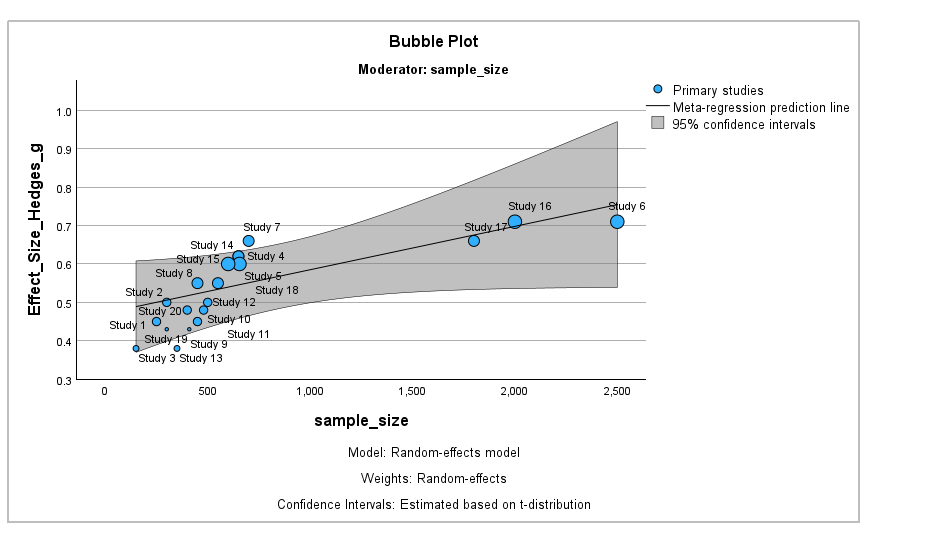
10. What is used for Bubble Plot in Meta-regression Analysis

A bubble plot is a visual tool in SPSS that helps display the relationship between an effect size and a moderator variable in meta-regression:

• The x-axis represents the moderator (factor or covariate).

• The y-axis shows the effect size (e.g., Hedge’s g or log odds).

• The size of each bubble reflects the weight of each study (usually inverse of variance).

It helps detect patterns such as linear trends, potential outliers, and effect modification. This plot is especially useful for continuous moderators (covariates), giving a quick visual summary of the regression relationship across studies.

11. What are the Assumptions of Meta-regression Analysis?

Meta-regression shares many assumptions with classical linear regression. Key assumptions include:

• Independence of studies: Each study should contribute independent data points.

• Linear relationship: The association between moderators and effect size should be linear.

• Homogeneity of variance (Homoscedasticity): The variance of effect sizes should be stable across values of the moderator.

• Normality of residuals: The residuals from the model should follow a normal distribution.

• Adequate number of studies: To avoid overfitting, the number of studies should exceed the number of predictors.

Violations can lead to biased coefficients, unreliable inferences, and inflated Type I error rates.

12. An Example for Meta-regression Analysis

To illustrate how meta-regression works in SPSS, let’s consider a meta-analysis of 20 medical studies evaluating the effectiveness of an intervention on reducing anxiety symptoms. The standardized mean differences (Hedges’ g) were used as the effect size metric. Each study also reported its variance and sample size. We aim to explore whether sample size (a continuous variable) predicts the observed effect sizes across studies.

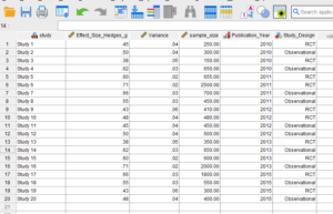
In this context, Hedges_g is the dependent variable, and sample_Size is the continuous moderator. Additionally, a categorical moderator Study_Design (RCT vs Observational) can be used for subgroup or interaction exploration. In the next section, we will show how to perform this meta-regression in SPSS using the meta-analysis module

Step by Step: Running Meta-Regression Analysis in SPSS Statistics

Let’s embark on a step-by-step guide on performing the meta-regerssion analysis using SPSS

To perform meta-regression analysis in SPSS:

1. STEP: Go to Analyze → Meta Analysis → Meta Regression.

2. STEP: Choose the appropriate input:

• Effect size variable (e.g., Hedges’ g)

• Standard error variable

• Covariates or factors as moderators.

3. STEP: In the Inference tab:

• Choose between Fixed effects or Random effects.
• Select the estimator (e.g., REML, DL, Sidik-Jonkman).
• Set standard error adjustment (e.g., Knapp-Hartung).

4. STEP: In the Print tab:

• Check Model Coefficient Test.

5. STEP: In the Plot tab:

• Check Model Bubble Predictor.

5. STEP: Click OK to run the analysis.

SPSS will produce output with pooled estimates, heterogeneity statistics, and visualizations.

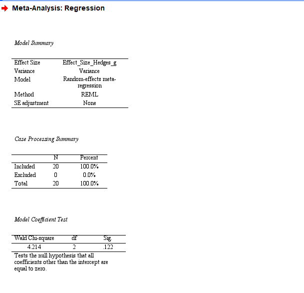
14. How to Interpret SPSS Output of Meta-Regression

After running a meta-regression in SPSS, the key output tables help determine whether the moderator variable (in this case, Sample_Size) significantly explains variability in the observed effect sizes.

• Model Coefficients Table: This shows the regression coefficient (B), standard error, test statistic, confidence interval, and p-value for each predictor. A statistically significant p-value (typically < .05) for the moderator suggests that it has a meaningful relationship with the effect size.

• Intercept: The intercept indicates the expected effect size when the moderator equals zero. Although not always substantively interpretable, it’s a necessary part of the model.

• Residual Heterogeneity (τ²): A reduction in residual heterogeneity compared to a model without moderators indicates that the moderator helps explain between-study variability.

• Test for Residual Heterogeneity (Q_E): This test assesses how much heterogeneity remains after accounting for the moderator. A non-significant result suggests the moderator adequately explains most of the heterogeneity.

• R² analog: This value, if reported, gives an idea of how much of the between-study variance is accounted for by the moderator.

15. How to Report Results of Meta-Regression in APA Style

When reporting meta-regression results in APA 7 style, include the following:

• A brief statement of the regression objective and variables

• Number of studies and the total sample size

• The method used (e.g., random-effects model with REML estimation)

• The regression coefficient (B), 95% confidence interval, and p-value

• Information about residual heterogeneity (Q_E, τ²)

• Optional: mention the variance explained (R² analog) if available

Get Help For Your SPSS Analysis

Embark on a seamless research journey with SPSSAnalysis.com, where our dedicated team provides expert data analysis assistance for students, academicians, and individuals. We ensure your research is elevated with precision. Explore our pages;

• Meta Analysis in Clinical Research
• Meta Analysis in Psychology
• Dissertation Help Statistics
• Dissertation Analysis Help
• Online Statistics Help
• SPSS Help by Subject Area: Psychology, Sociology, Nursing, Education, Medical, Healthcare, Epidemiology, Marketing 

Connect with us at SPSSAnalysis.com to empower your research endeavors and achieve impactful data analysis results. Get a FREE Quote Today!

PS: This guide is tailored for SPSS version 30, and for any variations, it’s recommended to refer to the software’s documentation for accurate and updated instructions.