Generalized Linear Model (GLM)

1. Introduction

Generalized Linear Model (GLM) extend traditional linear models by allowing for response variables that have error distributions other than a normal distribution. GLMs are highly flexible and can handle a wide range of data types, making them a powerful tool for many statistical analyses. By specifying a link function and a distribution from the exponential family, GLMs allow you to model relationships between the dependent and independent variables in non-normal data situations.

SPSS provides an accessible platform for conducting Generalized Linear Model, allowing users to analyse continuous, categorical, and count data with ease. In this blog post, we will explore what GLM is, their uses, and how to implement them in SPSS, making statistical analysis simpler for researchers.

2. What is the Generalized Linear Model in Statistics?

The Generalized Linear Model is a statistical framework that generalises linear regression models by allowing the dependent variable to follow distributions other than the normal distribution. In a traditional linear regression model, the relationship between the independent variables and the dependent variable assumes that the residuals are normally distributed. However, GLMs remove this assumption and extend the applicability to other types of data distributions, such as binomial, Poisson, and gamma distributions.

A key feature of GLMs is the use of a link function, which relates the linear predictor (the combination of independent variables) to the mean of the distribution of the dependent variable. This flexibility makes GLMs appropriate for handling diverse types of data and models such as logistic regression, Poisson regression, and gamma regression.

3. What is the Generalized Linear Model Used For?

Generalized Linear Models are widely used in fields such as epidemiology, social sciences, and economics, where data do not always follow normal distributions. GLMs are particularly valuable when analysing binary outcomes (e.g., success/failure), count data (e.g., the number of occurrences of an event), or proportional data (e.g., percentage of success). For instance, logistic regression, a type of GLM, is commonly used to model the probability of a binary outcome, while Poisson regression is used to model count data.

Researchers use GLMs to predict outcomes, assess relationships between variables, and control for confounders in non-normal data settings. With GLMs, one can model different types of response variables in a unified framework, making them highly versatile for real-world data that doesn’t meet the assumptions of traditional linear models.

3a. Type of Distribution

• Binomial: Models binary outcomes (e.g., success/failure, yes/no). It is often used in logistic regression and is appropriate when the dependent variable has two categories.
• Negative Binomial: Used for overdispersed count data, where the variance is greater than the mean. It is a generalisation of the Poisson distribution and allows for more flexibility in handling data with excess variability.
• Poisson: Used for modelling count data (e.g., the number of occurrences of an event). It assumes that the mean and variance are equal, making it ideal for rare event counts.
• Gamma: Used for continuous, positive data with a skewed distribution. It is often applied when modelling time to event or expenditure data where the outcome is strictly positive.
• Multinomial: Extends the binomial distribution to outcomes with more than two categories. It is suitable when the dependent variable represents multiple unordered categories.
• Normal: Assumes a continuous dependent variable that follows a normal (Gaussian) distribution. This is used in traditional linear regression models.

3b. Link Function 

• Identity: The simplest link function, where the predicted values are directly related to the linear predictor without any transformation. It is commonly used in linear regression.
• Log: The log link function transforms the predicted values using the natural logarithm, making it suitable for non-negative dependent variables. It is often used in Poisson regression for count data.
• Power: Transforms the dependent variable using an exponent. The power link is useful when relationships between variables follow a non-linear pattern and can adjust the transformation by choosing different power values.

3c. Scale Parameter Method

• MLE (Maximum Likelihood Estimation): Estimates the scale parameter by maximising the likelihood of the observed data, leading to more accurate model fitting.
• Deviance: Measures the goodness-of-fit of the model by comparing the observed and predicted values. It is often used when the goal is to assess how well the model explains the variability in the data.
• Pearson Chi-Square: Uses the Pearson residuals to calculate the scale parameter, which assesses the discrepancy between observed and expected frequencies in categorical data.
• Fixed Value: Sets the scale parameter to a constant value defined by the user. This method is used when the scale is known or needs to be constrained for specific modelling purposes.

3d. Choosing Appropriate Model Types For GLM

• Scale Response:
  • Linear: Models a continuous outcome with a normal distribution, assuming a direct relationship between predictors and the response.
  • Gamma with Log Link: Used for positive, skewed continuous data, such as time to event or cost data. The log link ensures that predictions remain positive.
• Ordinal Response:
  • Ordinal Logistic: Models ordered categorical outcomes where the categories have a meaningful ranking (e.g., strongly disagree to strongly agree). The model estimates the cumulative odds of being in or below a category.
  • Ordinal Probit: Similar to ordinal logistic, but assumes a normal distribution for the latent variable underlying the ordinal categories, making it useful when the assumption of proportional odds holds.
• Counts:
  • Poisson Loglinear: Models count data, assuming the number of events follows a Poisson distribution. It uses a log link to relate the predictors to the expected count.
  • Negative Binomial with Log Link: Extends the Poisson model to account for overdispersion, where the variance exceeds the mean, making it suitable for data with extra variability.
• Binary Response:
  • Binary Logistic: Used for modelling binary outcomes (e.g., success/failure). It estimates the log-odds of the event occurring and is widely used for classification problems.
  • Binary Probit: Similar to logistic regression but assumes a normal distribution for the latent variable underlying the binary response. It is often used when the relationship between variables is assumed to be cumulative.
  • Interval-Censored Survival: Models the time to an event when the exact time is unknown but lies within a known interval, useful in medical and reliability studies.

4. Explain the Differences Between GLM vs Regression vs ANOVA

Understanding the distinctions between Generalized Linear Models (GLM), regression, and ANOVA is essential for choosing the correct method for your analysis. Each of these approaches has specific applications depending on the type of data and the relationship being investigated. While all these methods help analyse relationships between variables, they do so under different assumptions and data structures.

The following points outline the key differences among these three statistical techniques:

• Generalized Linear Model (GLM): Extends linear regression by allowing for different types of distributions (e.g., binomial, Poisson) and incorporates link functions to model the response variable.
• Linear Regression: Models the relationship between a continuous dependent variable and one or more independent variables under the assumption of normally distributed residuals.
• ANOVA (Analysis of Variance): Compares the means of different groups to determine if there are significant differences among them. It is a special case of linear regression with categorical independent variables.

5. Explain Differences Among GLM, GLMM, and LMM

Generalized Linear Models (GLM), Generalized Linear Mixed Models (GLMM), and Linear Mixed Models (LMM) are all powerful tools for analysing data. However, they differ in how they handle different types of data and account for complexities in the data structure. GLMs are ideal when observations are independent, but in cases where data has a hierarchical structure or repeated measures, GLMMs or LMMs are more appropriate.

Below are the differences between GLM, GLMM, and LMM:

• Generalized Linear Model (GLM): Models non-normal response variables using a link function and assumes independence of observations.
• Generalized Linear Mixed Model (GLMM): Extends GLMs by incorporating random effects to account for correlations or hierarchical data structures.
• Linear Mixed Model (LMM): Models normally distributed continuous data with both fixed and random effects, used when data have grouped or repeated measures.

6. What are the Assumptions of the Generalized Linear Models?

Like any statistical model, Generalized Linear Models (GLMs) rely on several key assumptions that must be met to ensure valid results. By understanding these assumptions, researchers can better assess whether their data is suitable for GLMs and whether the results are reliable. Failing to meet these assumptions may lead to incorrect interpretations and results.

The following assumptions are fundamental for GLMs:

• The dependent variable follows a distribution from the exponential family (e.g., binomial, Poisson).
• The relationship between the dependent variable and the independent variables is defined by a link function.
• The observations must be independent.
• The model should not exhibit overdispersion (variance much larger than the mean).
• The error terms follow the distribution assumed by the model (e.g., Poisson for count data).

7. What is the Hypothesis of the Generalized Linear Models?

• Null Hypothesis (H₀): There is no relationship between the independent variables and the dependent variable (i.e., the regression coefficients for the independent variables are equal to zero).
• Alternative Hypothesis (H₁): There is a significant relationship between the independent variables and the dependent variable (i.e., at least one regression coefficient is not equal to zero).

Rejecting the null hypothesis indicates that the independent variables significantly predict the dependent variable.

8. An Example of the Generalized Linear Models

Consider a study that investigates the factors associated with the number of doctor visits in a year. The response variable (number of visits) follows a Poisson distribution because it counts the occurrences of an event. Independent variables might include age, gender, income, and health status. A Generalized Linear Model can be applied to model the relationship between these predictors and the count of doctor visits.

The researcher would use a Poisson regression model (a type of GLM) with a log link function, which is suitable for count data. The model would estimate how each factor influences the number of visits, controlling for other variables.

Step by Step: Running Generalized Linear Model in SPSS Statistics

Let’s embark on a step-by-step guide on performing the GLM using SPSS

1. STEP: Load Data into SPSS

Commence by launching SPSS and loading your dataset, which should encompass the variables of interest – a categorical independent variable. If your data is not already in SPSS format, you can import it by navigating to File > Open > Data and selecting your data file.

2. STEP: Access the Analyze Menu

In the top menu, In SPSS, click on Analyse > Generalized Linear Models > Generalized Linear Models.

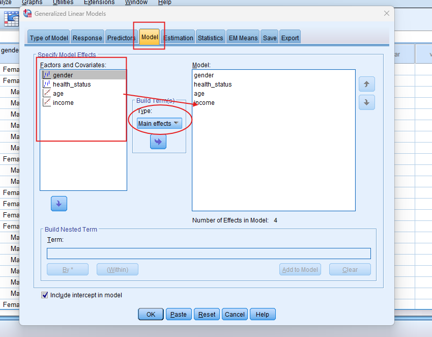
3. STEP: Specify Variables 

• Define the model: Select the dependent variable and choose the distribution that matches the data (e.g., binomial, Poisson).
• Choose the link function: Select the appropriate link function for your data, such as log for Poisson or logit for binary data.
• Specify predictors: Add the independent variables to the model.

4. STEP: Generate SPSS Output

• Click ‘OK’ after selecting your variables and method. SPSS will run the analysis and generate output tables and survival curves.

Note: Conducting a Generalized Linear Model in SPSS provides a robust foundation for understanding the key features of your data. Always ensure that you consult the documentation corresponding to your SPSS version, as steps might slightly differ based on the software version in use. This guide is tailored for SPSS version 25, and for any variations, it’s recommended to refer to the software’s documentation for accurate and updated instructions.

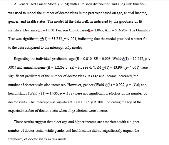
11. How to Interpret SPSS Output of Generalized Linear Model

SPSS will generate output, including Model Information, Case Processing Summary, Goodness of Fit, Omnibus Test, Tests of model effects, and parameter estimates.

• Model Information Table: Describes the model, the distribution used, and the link function.
• Goodness-of-Fit Table: Provides statistics to assess how well the model fits the data (e.g., Pearson Chi-Square).
• Parameter Estimates Table: Displays the regression coefficients, standard errors, and significance values for each predictor.
• Omnibus or Likelihood Ratio Tests: Shows whether the predictors are significant based on likelihood ratio Chi-Square tests.

12. How to Report Results of Generalized Linear Model in APA

Reporting the results of GLM in APA (American Psychological Association) format requires a structured presentation. Here’s a step-by-step guide in list format:

• Introduction: Briefly describe the purpose of the analysis and the theoretical background.
• Method: Detail the data collection process, variables used, and the model specified.
• Results: Present the parameter estimates with their standard errors, and significance levels.
• Figures and Tables: Include relevant plots and tables, ensuring they are properly labelled and referenced.
• Discussion: Interpret the results, highlighting the significance of the findings and their implications.
• Conclusion: Summarise the main points and suggest potential areas for further research.

Get Support For Your SPSS Data Analysis

Embark on a seamless research journey with SPSSAnalysis.com, where our dedicated team provides expert data analysis assistance for students, academicians, and individuals. We ensure your research is elevated with precision. Explore our pages;

• Biostatistical Modeling Expert
• Statistical Methods for Clinical Studies
• Epidemiological Data Analysis
• Biostatistical Support for Researchers
• Clinical Research Data Analysis
• Medical Data Analysis Expert
• Biostatistics Consulting
• Healthcare Data Statistics Consultant

• SPSS Help by Subjects Area: Psychology, Sociology, Nursing, Education, Medical, Healthcare, Epidemiology, Marketing 

Connect with us at SPSSAnalysis.com to empower your research endeavors and achieve impactful data analysis results. Get a FREE Quote Today!