Canonical Correlation Analysis in SPSS

Introduction

Canonical Correlation Analysis (CCA) stands as a powerful multivariate statistical technique used to explore the relationships between two sets of variables simultaneously. In the realm of data analysis, CCA goes beyond traditional methods, allowing researchers to unravel intricate patterns of association between sets of variables that may be interrelated in complex ways. This blog post aims to demystify Canonical Correlation Analysis in SPSS, providing a comprehensive overview of its applications, assumptions, and practical steps for interpretation.

Whether you are engaged in social science research, market analysis, or any field requiring a nuanced understanding of variable relationships, CCA can be a valuable tool in your analytical toolkit. As we delve into the intricacies of this method, we will explore how CCA enables researchers to uncover hidden connections within their datasets, contributing to a deeper understanding of the underlying structures governing diverse sets of variables.

What are the 5 Correlation Analyses?

Correlation Analysis offers various methods to explore associations between variables. Besides the commonly used Pearson Correlation, others include Spearman’s Rho rank order, Kendall’s Tau, Partial Correlation, and Canonical Correlation.

1. Pearson Correlation Analysis

• Description: Measures the linear relationship between two continuous variables.
• Applicability: Best suited for variables with a linear association and normally distributed data.
• Range: Correlation coefficient (r) ranges from -1 to 1.
• Interpretation: Positive values indicate a positive linear relationship, negative values indicate a negative linear relationship, and 0 implies no linear relationship.

2. Spearman Rank-Order Correlation

• Description: Non-parametric measure assessing the monotonic relationship between two variables.
• Applicability: Suitable for ordinal data or when assumptions of normality are violated.
• Procedure: Converts data into ranks and compute the correlation based on the rank differences.
• Interpretation: The correlation coefficient (rho) ranges from -1 to 1, with a similar interpretation to Pearson.

3. Kendall’s Tau

• Description: Non-parametric measure assessing the strength and direction of a monotonic relationship.
• Applicability: Similar to Spearman, suitable for ordinal data and non-normally distributed data.
• Procedure: Measures the number of concordant and discordant pairs in the data.
• Interpretation: Kendall’s Tau (τ) ranges from -1 to 1, with 0 indicating no association and values towards -1 or 1 indicating stronger associations.

4. Partial Correlation

• Description: Examines the relationship between two variables while controlling for the influence of one or more additional variables.
• Applicability: Useful when there is a need to isolate the direct relationship between two variables.
• Procedure: Calculates the correlation between two variables after removing the shared variance with the control variable(s).
• Interpretation: Provides insights into the unique contribution of each variable to the correlation.

5. Canonical Correlation

• Description: Assesses the association between two sets of variables.
• Applicability: Useful when dealing with multiple sets of variables simultaneously.
• Procedure: Maximizes the correlation between linear combinations of variables from each set.
• Interpretation: Provides information on the overall relationship between sets of variables, producing canonical correlation coefficients.

Understanding the characteristics and applications of each correlation analysis method equips researchers with a versatile toolkit for exploring diverse data scenarios.

Definition: Canonical Correlation

At its core, Canonical Correlation Analysis seeks to examine the relationships between two sets of variables (X and Y) by identifying linear combinations (canonical variates) within each set that exhibit the highest correlation across sets. In other words, CCA helps researchers understand how changes in one set of variables correspond to changes in another. This is particularly useful when dealing with multiple dependent variables and their interdependencies, providing a holistic view of the associations present in complex datasets. Canonical Correlation Analysis is well-suited for scenarios where the researcher aims to explore the simultaneous influence of multiple factors on an outcome, making it a versatile and insightful method for a range of research questions. Now, let’s explore the assumptions that underlie the application of Canonical Correlation Analysis.

Assumption of Canonical Correlation Analysis

Canonical Correlation Analysis, like many statistical methods, operates under certain assumptions to ensure the validity and reliability of its results. Here are the key assumptions that should be considered when employing CCA:

• Linearity: The relationships between variables in both sets should be linear. Non-linear associations may compromise the accuracy of canonical correlation results.
• Multivariate Normality: The variables in both sets should follow a multivariate normal distribution. Departures from normality might affect the precision of canonical correlation coefficients.
• No Perfect Multicollinearity: There should be no perfect linear relationship among variables within each set. Multicollinearity can lead to unstable estimates and inflated standard errors.
• Homogeneity of Variance-Covariance Matrices: The variance-covariance matrices of both sets should be homogenous. This implies that the variability within each set should be relatively consistent across all levels of the other set.
• Random Sampling: The data should be collected through a random sampling process to ensure that the results can be generalized to the broader population.

Understanding and addressing these assumptions are crucial for obtaining meaningful and valid results from Canonical Correlation Analysis using SPSS Statistics. Now, let’s illustrate the application of CCA with a practical example.

Example of Canonical Correlation

Consider a study examining the relationship between socioeconomic status (SES) and academic achievement. The researcher is interested in understanding how a set of socioeconomic variables (e.g., income, education level) is correlated with academic performance variables (e.g., grades, test scores). Canonical Correlation Analysis can reveal the canonical variates representing the most significant patterns of association between these two sets of variables. This example demonstrates how CCA can unveil complex relationships, providing valuable insights for researchers in diverse fields.

As we progress, we will guide you through the steps of performing Canonical Correlation Analysis in SPSS, offering practical insights into interpretation and reporting. This knowledge will empower you to harness the full potential of Canonical Correlation Analysis for your research endeavors.

Step by Step: Running Canonical Correlation in SPSS Statistics

Now, let’s delve into the step-by-step process of conducting the Canonical Correlation using SPSS.  Here’s a step-by-step guide on how to perform a Canonical Correlation Analysis in SPSS:

1. STEP: Load Data into SPSS

Commence by launching SPSS and loading your dataset, which should encompass the variables of interest – a categorical independent variable. If your data is not already in SPSS format, you can import it by navigating to File > Open > Data and selecting your data file.

2. STEP: Access the Analyze Menu

In the top menu, locate and click on “Analyze.” Within the “Analyze” menu, navigate to “Correlate” and choose ” Bivariate” Analyze > Correlate> Canonical Correlation

3. STEP: Choose Variables

– Move the variables you want to include in each set to the appropriate boxes (Set 1 and Set 2).

4. STEP: Generate SPSS Output

Once you have specified your variables and chosen options, click the “OK” button to perform the analysis. SPSS will generate a comprehensive output, including the requested frequency table and chart for your dataset.

Executing these steps initiates the Canonical Correlation Analysis in SPSS, allowing researchers to assess the impact of the teaching method on students’ test scores while considering the repeated measures. In the next section, we will delve into the interpretation of SPSS output for Canonical Correlation Analysis.

Note

Conducting a Canonical Correlation Analysis in SPSS provides a robust foundation for understanding the key features of your data. Always ensure that you consult the documentation corresponding to your SPSS version, as steps might slightly differ based on the software version in use. This guide is tailored for SPSS version 25, and any variations, it’s recommended to refer to the software’s documentation for accurate and updated instructions.

How to Interpret SPSS Output of Canonical Correlation Analysis

Once Canonical Correlation Analysis has been conducted in SPSS, the output provides valuable information about the relationships between the sets of variables. Here are key components of the SPSS output and how to interpret them:

• Canonical Correlation Coefficients: These coefficients indicate the strength and direction of the relationship between the canonical variates in the two sets. Higher values suggest stronger associations.
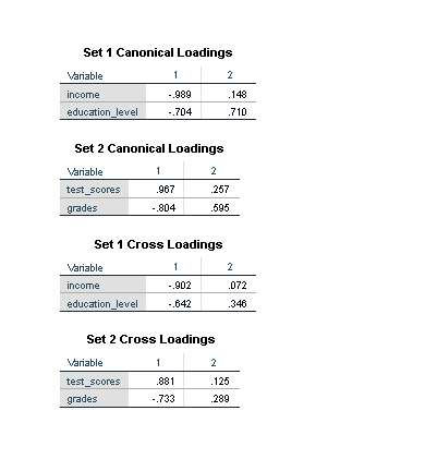
• Canonical Loadings: Loadings represent the correlations between the original variables and the canonical variates. High loadings indicate variables that contribute significantly to the canonical correlation.
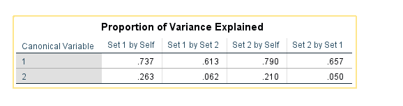
• Redundancy Index: The redundancy index represents the proportion of variance in one set of variables explained by the other set. It ranges from 0% (no shared variance) to 100% (complete shared variance).
• Eigenvalues: Eigenvalues indicate the proportion of variance in the canonical variates. Larger eigenvalues suggest more substantial canonical correlation structures.
• Wilks’ Lambda: This test assesses the overall significance of canonical correlation. A significant Wilks’ Lambda suggests that at least one pair of canonical variates is significantly related.

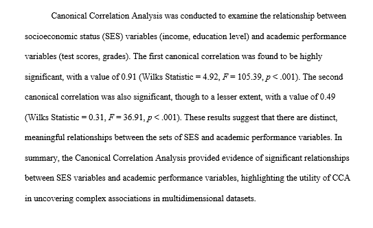
How to Report Results of Canonical Correlation Analysis in APA

When reporting the results of Canonical Correlation Analysis in APA format, it is essential to provide clear and concise information.

By following these guidelines, you can effectively communicate the results of Canonical Correlation Analysis in a format consistent with APA standards. This ensures that your research is presented clearly and professionally, facilitating understanding and replication by fellow researchers.

Get Help For Your SPSS Analysis

Embark on a seamless research journey with SPSSAnalysis.com, where our dedicated team provides expert data analysis assistance for students, academicians, and individuals. We ensure your research is elevated with precision. Explore our pages;

• SPSS Data Analysis Help – SPSS Helper,
• Quantitative Analysis Help,
• Qualitative Analysis Help,
• SPSS Dissertation Analysis Help,
• Dissertation Statistics Help,
• Statistical Analysis Help,
• Medical Data Analysis Help.

Connect with us at SPSSAnalysis.com to empower your research endeavors and achieve impactful results. Get a Free Quote Today!