Backward Regression in SPSS

Introduction

Embark on a journey into the heart of statistical modeling with our exploration of Backward Regression in SPSS. In the ever-evolving landscape of data analysis, Backward Regression stands out as a powerful technique for refining predictive models. This blog post is your guide to unravel the intricacies of Backward Regression, offering insights and practical knowledge for researchers and analysts alike.

Whether you are navigating complex datasets or seeking optimal variable selection, we will navigate through the fundamentals, applications, and the step-by-step process of implementing Backward Regression in SPSS. This exploration is your key to unlocking the potential of your data, and enhancing your ability to make informed decisions based on robust statistical analysis.

Definition: Backward Regression

Backward Regression is a method nested within the realm of multiple linear regression. It serves as a systematic approach to building models by iteratively removing the least statistically significant predictor variables. The process commences with an initial model containing all relevant predictors, and secondly, it strategically eliminates variables that contribute the least to the model’s explanatory power. Backward Regression is akin to sculpting a model to its most essential elements. It ensures that only the most impactful predictors remain, thereby simplifying the model while retaining its predictive accuracy. This approach is particularly beneficial when dealing with datasets rich in variables, enabling analysts to focus on the core contributors to the dependent variable’s variance. As we dive into the Backward Regression equation, the elegance of its simplicity and efficiency will become apparent, highlighting its significance in the arsenal of statistical techniques.

Backward Regression Equation

Now, let’s navigate through the mechanics of the Backward Regression Equation. Firstly, envision the initial model containing all relevant predictors:

• [ Y = b_0 + b_1X_1 + b_2X_2 + …. + b_nX_n ]

Secondly, the Backward Regression process begins by iteratively removing the least statistically significant predictor variable. Let’s denote the least impactful variable as (X_n). The equation adapts as follows:

• [ Y = b_0 + b_1X_1 + b_2X_2 + …+ b_{n-1}X_{n-1} ]

The algorithm continues this iterative process, sequentially removing the least significant predictors until reaching the final Backward Regression Equation:

• [ Y = b_0 + b_1X_1 + b_2X_2 + …. + b_kX_k ]

Here, (b_0, b_1, b_2, …., b_k) represent the intercept and the coefficients for the selected significant predictor variables (X_1, X_2, …, X_k).

The elegance of the Backward Regression Equation lies in its simplicity, providing a streamlined representation of the model while retaining robust predictive power. By systematically pruning less impactful variables, this method enhances interpretability and ensures that the resulting model focuses on the essential contributors to the dependent variable. Understanding the mechanics of the Backward Regression Equation empowers analysts to refine their models efficiently, extracting meaningful insights from complex datasets.

 Assumption of Backward Linear Regression

Before diving into Backward Linear Regression analysis, it’s crucial to be aware of the underlying assumptions that bolster the reliability of the results.

• Linearity: Assumes a linear relationship between the dependent variable and all independent variables. The model assumes that changes in the dependent variable are proportional to changes in the independent variables.
• Independence of Residuals: Assumes that the residuals (the differences between observed and predicted values) are independent of each other. The independence assumption is crucial to avoid issues of autocorrelation and ensure the reliability of the model.
• Homoscedasticity: Assumes that the variability of the residuals remains constant across all levels of the independent variables. Homoscedasticity ensures that the spread of residuals is consistent, indicating that the model’s predictions are equally accurate across the range of predictor values.
• Normality of Residuals: Assumes that the residuals follow a normal distribution. Normality is essential for making valid statistical inferences and hypothesis testing. Deviations from normality may impact the accuracy of confidence intervals and p-values.
• No Perfect Multicollinearity: Assumes that there is no perfect linear relationship among the independent variables. Perfect multicollinearity can lead to unstable estimates of regression coefficients, making it challenging to discern the individual impact of each predictor.

These assumptions collectively form the foundation of Backward Regression analysis. Ensuring that these conditions are met enhances the validity and reliability of the statistical inferences drawn from the model. In the subsequent sections, we will delve into hypothesis testing in Backward Regression, provide practical examples, and guide you through the step-by-step process of performing and interpreting Backward Regression analyses using SPSS.

Hypothesis of Backward Regression

The hypothesis in Backward Regression revolves around the significance of the regression coefficients. Each coefficient corresponds to a specific predictor variable, and the hypothesis tests whether each predictor has a significant impact on the dependent variable.

• Null Hypothesis (H0): The regression coefficients for all independent variables are simultaneously equal to zero.
• Alternative Hypothesis (H1): At least one regression coefficient for an independent variable is not equal to zero.

The hypothesis testing in Backward Regression revolves around assessing whether the collective set of independent variables has a statistically significant impact on the dependent variable. The null hypothesis suggests no overall effect, while the alternative hypothesis asserts the presence of at least one significant relationship. This testing framework guides the evaluation of the model’s overall significance, providing valuable insights into the joint contribution of the predictor variables.

Example of Backward Regression

To illustrate the concepts of Backward Regression, let’s consider an example. Imagine you are studying the factors influencing house prices, with predictors such as square footage, number of bedrooms, and distance to the city centre. By applying Backward Regression, you can model how these factors collectively influence house prices.

Through this example, you’ll gain practical insights into how Backward Regression can untangle complex relationships and offer a comprehensive understanding of the factors affecting the dependent variable.

Step by Step: Running Backward Regression in SPSS Statistics

Now, let’s delve into the step-by-step process of conducting the Backward Regression using SPSS Statistics.  Here’s a step-by-step guide on how to perform a Backward Regression in SPSS:

1. STEP: Load Data into SPSS

Commence by launching SPSS and loading your dataset, which should encompass the variables of interest – a categorical independent variable. If your data is not already in SPSS format, you can import it by navigating to File > Open > Data and selecting your data file.

2. STEP: Access the Analyze Menu

In the top menu, locate and click on “Analyze.” Within the “Analyze” menu, navigate to “Regression” and choose ” Linear” Analyze > Regression> Linear

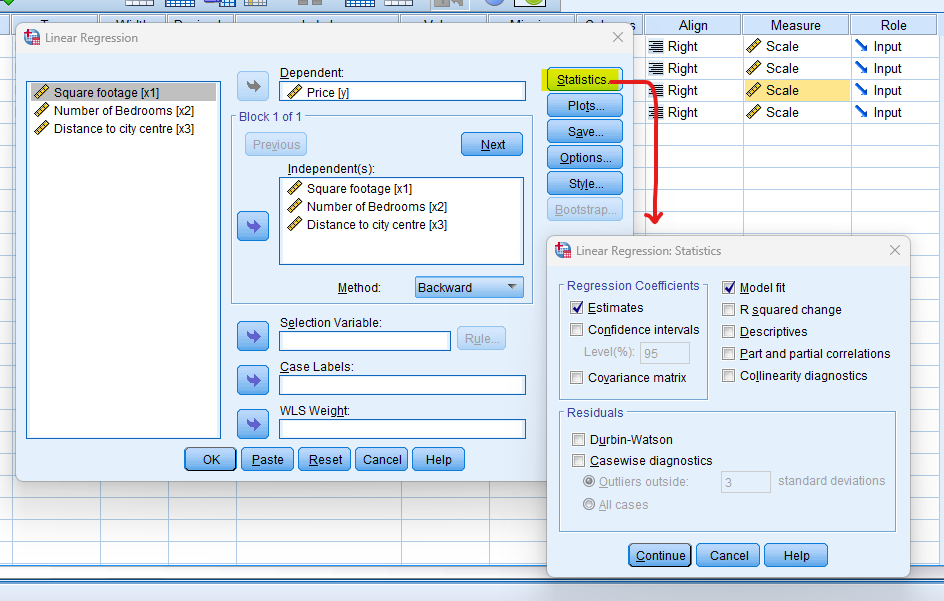
3. STEP: Choose Variables

A dialogue box will appear. Move the dependent variable (the one you want to predict) to the “Dependent” box and the independent variables to the “Independent” box.

In the Method section, Choose “Backward”

4. STEP: Generate SPSS Output

Once you have specified your variables and chosen options, click the “OK” button to perform the analysis. SPSS will generate a comprehensive output, including the requested frequency table and chart for your dataset.

Executing these steps initiates the Backward Regression in SPSS, allowing researchers to assess the impact of the teaching method on students’ test scores while considering the repeated measures. In the next section, we will delve into the interpretation of SPSS output for Backward Regression.

Note

Conducting a Backward Regression in SPSS provides a robust foundation for understanding the key features of your data. Always ensure that you consult the documentation corresponding to your SPSS version, as steps might slightly differ based on the software version in use. This guide is tailored for SPSS version 25, and for any variations, it’s recommended to refer to the software’s documentation for accurate and updated

How to Interpret SPSS Output of Backward Regression

Deciphering the SPSS output of Backward Regression is a crucial skill for extracting meaningful insights. Let’s focus on three tables in SPSS output;

Model Summary Table

• R (Correlation Coefficient): This value ranges from -1 to 1 and indicates the strength and direction of the linear relationship. A positive value signifies a positive correlation, while a negative value indicates a negative correlation.
• R-Square (Coefficient of Determination): Represents the proportion of variance in the dependent variable explained by the independent variable. Higher values indicate a better fit of the model.
• Adjusted R Square: Adjusts the R-squared value for the number of predictors in the model, providing a more accurate measure of goodness of fit.

ANOVA Table

• F (ANOVA Statistic): Indicates whether the overall regression model is statistically significant. A significant F-value suggests that the model is better than a model with no predictors.
• df (Degrees of Freedom): Represents the degrees of freedom associated with the F-test.
• P values: The probability of obtaining the observed F-statistic by random chance. A low p-value (typically < 0.05) indicates the model’s significance.

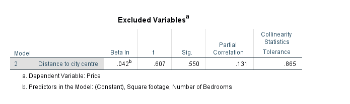
Coefficient Table

• Unstandardized Coefficients (B): Provides the individual regression coefficients for each predictor variable.
• Standardized Coefficients (Beta): Standardizes the coefficients, allowing for a comparison of the relative importance of each predictor.
• t-values: Indicate how many standard errors the coefficients are from zero. Higher absolute t-values suggest greater significance.
• P values: Test the null hypothesis that the corresponding coefficient is equal to zero. A low p-value suggests that the predictors are significantly related to the dependent variable.

Understanding these tables in the SPSS output is crucial for drawing meaningful conclusions about the strength, significance, and direction of the relationship between variables in a Backward Regression analysis.

 How to Report Results of Backward Regression in APA

Effectively communicating the results of Backward Regression in compliance with the American Psychological Association (APA) guidelines is crucial for scholarly and professional writing

• Introduction: Begin the report with a concise introduction summarizing the purpose of the analysis and the relationship being investigated between the variables.
• Assumption Checks: If relevant, briefly mention the checks for assumptions such as linearity, independence, homoscedasticity, and normality of residuals to ensure the robustness of the analysis.
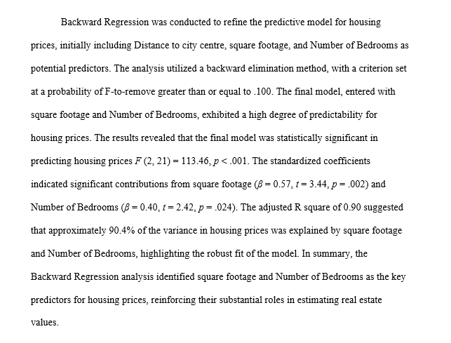
• Significance of the Model: Comment on the overall significance of the model based on the ANOVA table. For example, “The overall regression model was statistically significant (F = [value], p = [value]), suggesting that the predictors collectively contributed to the prediction of the dependent variable.”
• Regression Equation: Present the Regression equation, highlighting the intercept and regression coefficients for each predictor variable.
• Coefficients and Significance: Discuss the significance of each regression coefficient, emphasizing how each predictor contributes to the variation in the dependent variable.
• Interpretation of Coefficients: Interpret the coefficients, focusing on the slope (b1..bn) to explain the strength and direction of the relationship. Discuss how a one-unit change in the independent variable corresponds to a change in the dependent variable.
• R-squared Value: Include the R-squared value to highlight the proportion of variance in the dependent variable explained by the independent variables. For instance, “The R-squared value of [value] indicates that [percentage]% of the variability in [dependent variable] can be explained by the linear relationship with [independent variables].”
• Conclusion: Conclude the report by summarizing the key findings and their implications. Discuss any practical significance of the results in the context of your study.

Get Help For Your SPSS Analysis

Embark on a seamless research journey with SPSSAnalysis.com, where our dedicated team provides expert data analysis assistance for students, academicians, and individuals. We ensure your research is elevated with precision. Explore our pages;

• SPSS Data Analysis Help – SPSS Helper,
• Quantitative Analysis Help,
• Qualitative Analysis Help,
• SPSS Dissertation Analysis Help,
• Dissertation Statistics Help,
• Statistical Analysis Help,
• Medical Data Analysis Help.

Connect with us at SPSSAnalysis.com to empower your research endeavors and achieve impactful results. Get a Free Quote Today!