Structural Equation Modelling in SPSS AMOS

Introduction

Structural Equation Modelling (SEM) represents a powerful statistical technique used to test and estimate causal relationships using a combination of statistical data and qualitative causal assumptions. Researchers and analysts employ SEM to explore complex relationships among variables, making it essential in fields such as psychology, sociology, and business research. SEM allows for the simultaneous examination of multiple dependent and independent variables, offering a comprehensive approach to data analysis.

In this blog post, we delve into the intricacies of Structural Equation Modelling (SEM) in SPSS AMOS. We will cover fundamental concepts, the SEM framework, and various types of SEM. Additionally, we will discuss path diagram symbols, key assumptions, and hypothesis testing in SEM. By the end of this article, you will gain a thorough understanding of how to leverage SEM in SPSS AMOS to enhance your research and data analysis capabilities.

1. What is Structural Equation Modelling in SPSS AMOS?

Structural Equation Modelling (SEM) in SPSS AMOS is a statistical methodology that combines factor analysis and multiple regression analysis. This integration enables researchers to examine complex relationships among observed and latent variables. SEM in SPSS AMOS facilitates the creation of models that represent theoretical constructs and their relationships, providing a robust framework for testing hypotheses and theories.

SPSS AMOS (Analysis of Moment Structures) is a specialised software tool designed for SEM. It offers a user-friendly graphical interface, allowing users to draw path diagrams and specify models visually. Researchers can estimate and assess models efficiently, obtaining detailed outputs that help in the thorough evaluation of proposed models. By using SEM in SPSS AMOS, researchers can explore intricate data structures, ensuring comprehensive insights and rigorous data analysis.

2. Structural Equation Modelling: Some Definitions

• Observed Variable: An observed variable is a measurable variable in a study, directly recorded from respondents. It serves as a foundational element in SEM, representing tangible data points.
• Latent Variable: A latent variable is not directly observable but inferred from observed variables. These variables represent underlying constructs, such as intelligence or satisfaction.
• Exogenous Variable: Exogenous variables are independent variables within SEM, not influenced by other variables in the model. They serve as predictors or determinants of other variables.
• Endogenous Variable: Endogenous variables are dependent variables influenced by one or more exogenous variables. They act as outcomes or effects within the model.
• Measurement Model: The measurement model specifies the relationships between observed variables and their underlying latent constructs. It essentially forms the basis of factor analysis within SEM.
• Indicator: An indicator is an observed variable used to define a latent variable. Indicators are essential for the measurement of latent constructs.
• Factor: A factor represents a latent variable in the model, underlying the observed variables. Factors illustrate how observed data reflect abstract constructs.
• Loading: Loadings are coefficients that show the relationship strength between observed variables and their corresponding latent variables. Higher loadings indicate a stronger relationship.
• Structural Model: The structural model defines the relationships between latent variables. It shows how constructs interact and influence each other within the SEM framework.
• Regression Path: A regression path represents the directional influence between variables in the model. It depicts causal relationships and the flow of influence within SEM.

3. Types of Structural Equation Models

Structural Equation Modelling encompasses various types, each serving distinct purposes and involving different combinations of endogenous and exogenous variables, whether observed or latent. Understanding these types helps in selecting the appropriate model for specific research questions. The following diagram helps to choose an appropriate model for your research question;

• Simple Regression: Involves one exogenous (independent) and one endogenous (dependent) observed variable. It examines the direct influence of one variable on another.
• Multiple Regression: Consists of multiple exogenous observed variables predicting a single endogenous observed variable. It assesses the combined effect of several predictors on one outcome.
• Multivariate Analysis: Includes multiple endogenous observed variables influenced by multiple exogenous observed variables. This model evaluates the relationships among multiple predictors and outcomes simultaneously.
• Path Analysis: Focuses on observed variables, examining direct and indirect relationships among them. It explores causal paths without involving latent constructs.
• Confirmatory Factor Analysis (CFA): Investigates the measurement model by testing how well observed variables represent latent constructs. It confirms the factor structure hypothesised in the theory.
• Structural Regression: Combines CFA and path analysis, examining relationships between latent variables and their observed indicators. It integrates the measurement and structural models to assess complex relationships.

4. Path Diagram Symbols

• Latent Variable Symbol: Represented by circles or ellipses, latent variables are theoretical constructs not directly observed but inferred from measured variables. They signify underlying traits or factors.
• Observed Variable Symbol: Represented by rectangles or squares, observed variables are directly measured indicators. These symbols denote the data collected through surveys or experiments.

• Intercept Symbol: Intercepts, often represented by a triangle or a point, indicate the expected value of the dependent variable when all predictors are zero. It represents the baseline level of the variable.
• Path Symbol: Arrows depict paths, illustrating directional relationships between variables. A single-headed arrow signifies a unidirectional influence, while double-headed arrows indicate covariances or correlations.
• Covariance Symbol: Double-headed arrows between variables represent covariances or correlations, showing the degree to which two variables change together. They indicate mutual relationships without implying causation.

5. Visualising Structural Equation Modelling

The diagram illustrates a Structural Equation Model (SEM), highlighting the relationship between exogenous and endogenous latent variables and their measurement models. On the left, the x-side measurement model includes exogenous latent variables (circles) influencing observed indicators (rectangles). Arrows indicate loadings, showing the strength of each indicator’s relationship with its latent variable. Smaller circles and arrows denote residual variances, accounting for unexplained variance in the indicators.

Centrally, the structural model shows the regression path from the exogenous latent variable to the endogenous latent variable, representing a causal relationship. On the right, the y-side measurement model features the endogenous latent variable and its observed indicators. Loadings and residual variances are similarly depicted, highlighting the relationships and unexplained variances.

This diagram effectively captures the complexity of SEM, illustrating how latent variables influence observed indicators and interact within the structural model. Understanding these relationships is crucial for accurate SEM analysis.

6. Model Indices for Structural Equation Modelling (SEM)

Acceptable fit indices provide benchmarks for determining whether a structural equation model adequately fits the data. Generally, a good fit is indicated by a Chi-Square (Chisq) value that is non-significant, although this is sensitive to sample size. Goodness of Fit Index (GFI) and Adjusted Goodness of Fit Index (AGFI) values should exceed 0.90 for a good fit.

Comparative Fit Index (CFI) and Tucker-Lewis Index (TLI) values above 0.95 indicate an excellent fit, while values above 0.90 are considered acceptable. Root Mean Square Error of Approximation (RMSEA) values below 0.06 indicate a close fit, with values up to 0.08 representing a reasonable error of approximation. Standardized Root Mean Square Residual (SRMR) values less than 0.08 are generally indicative of a good model fit.

7. What are the Assumptions of Structural Equation Modelling?

• Linearity: The relationships among variables are linear.
• Normality: Variables are normally distributed.
• Independence: Observations are independent.
• Measurement Error: Measurement errors are uncorrelated.
• Model Specification: The model is correctly specified.
• Sample Size: Adequate sample size for reliable results.
• Multicollinearity: No perfect multicollinearity among exogenous variables.
• Identification: The model is identifiable, meaning a unique solution can be obtained.
• Model Fit: The model adequately fits the data.
• Path Coefficients: Path coefficients are stable across different samples.

8. What is the Hypothesis of SEM?

In SEM, researchers formulate hypotheses based on theoretical frameworks and prior research. A typical hypothesis might state that a latent variable significantly predicts an observed outcome. For example, one might hypothesise that emotional disorders significantly influence depression.

Hypotheses in SEM involve testing the significance of path coefficients, which represent the strength and direction of relationships. Researchers use SPSS AMOS to estimate these coefficients and test the hypotheses, examining empirical support for the theoretical model. This process helps validate the proposed relationships and refine theoretical constructs. By testing these hypotheses, researchers can draw conclusions about the nature and strength of the relationships within their data, ultimately contributing to a deeper understanding of the phenomena under study.

9. An Example of Structural Equation Modelling

Consider a study aiming to understand how emotional disorders influence depression among adults. Researchers propose a model where emotional disorders and depression are latent variables, each measured by five Likert-scale items. The study hypothesises that emotional disorders significantly predict levels of depression.

Firstly, researchers define the measurement model. For emotional disorders, the five Likert items might include questions like “I often feel anxious” and “I struggle with mood swings.” For depression, the items could be “I feel sad frequently” and “I have trouble enjoying activities.” These items serve as indicators of their respective latent constructs.

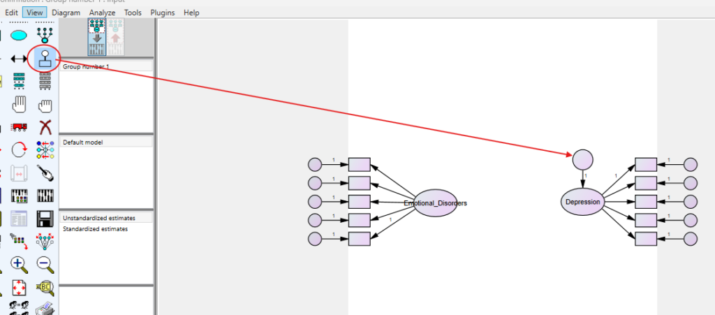
Using SPSS AMOS, researchers construct the model by specifying the relationships between the latent variables (emotional disorders and depression). The path diagram illustrates how emotional disorders, as a latent variable, influence depression. Researchers would then collect data, input it into SPSS, and use AMOS to estimate the model’s parameters. The output provides insights into how strongly emotional disorders impact depression, helping psychologists and mental health professionals develop better intervention strategies.

Step by Step: Running Structural Equation Analysis in SPSS AMOS

Let’s embark on a step-by-step guide on performing the Structural Equation Modelling in SPSS AMOS

1. Define Variables: Start by defining the observed and latent variables in your model. Here, the latent variables are emotional disorders and depression, each measured by five Likert-scale items.
2. Draw Path Diagram: Use AMOS’s graphical interface to draw the path diagram. Depict emotional disorders as a latent variable with arrows pointing to its five observed indicators. Similarly, depict depression with its five indicators. Draw an arrow from emotional disorders to depression to represent the hypothesised predictive relationship.
3. Specify Model: Input the paths and correlations between variables in the diagram. Ensure that each observed item correctly loads onto its respective latent construct.
4. Input Data: Load your dataset into SPSS and link it to AMOS.
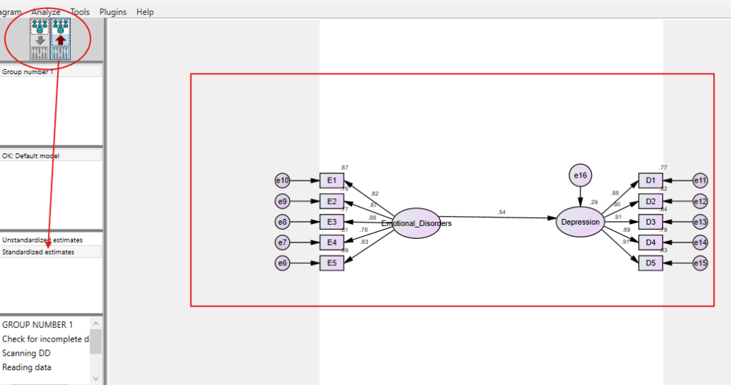
5. Estimate Model: Run the estimation process to obtain path coefficients and model fit indices.
6. Evaluate Fit: Check the goodness-of-fit indices, such as Chi-square, RMSEA, CFI, and TLI, to assess how well the model fits the data. Ensure the values meet acceptable thresholds.
7. Refine Model: Modify the model based on the fit indices and theoretical considerations if necessary.
8. Interpret Results: Analyse the output to understand the relationships and their significance.

How to Interpret SPSS AMOS Output of Structural Equation Modelling

When interpreting the SPSS AMOS output for a Structural Equation Analysis, focus on several key components. Firstly, examine the path coefficients, which indicate the strength and direction of the relationships between variables. Significant path coefficients suggest meaningful relationships, while non-significant ones may need re-evaluation. Secondly, review the goodness-of-fit indices, such as the Chi-square test, RMSEA, CFI, and TLI, to determine how well the model fits the data.

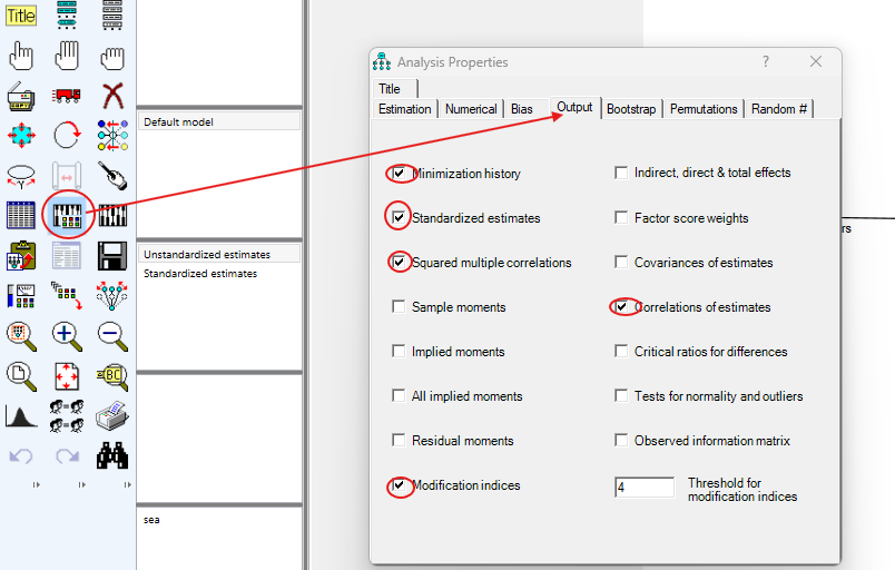
Additionally, consider the standardised residuals and modification indices. Standardised residuals help identify any discrepancies between observed and predicted values, pointing out areas where the model may not fit well. Modification indices suggest potential adjustments to improve model fit, such as adding or removing paths. By carefully analysing these outputs, researchers can validate their theoretical models and ensure robust conclusions.

How to Report Results of Structural Equation Modelling in APA

1. Model Description: Describe the theoretical model and the hypothesised relationships.
2. Data Collection: Explain the data collection process and sample characteristics.
3. Model Specification: Detail how the model was specified, including the paths and variables.
4. Goodness-of-Fit: Report the goodness-of-fit indices, including Chi-square, RMSEA, CFI, and TLI.
5. Path Coefficients: Present the path coefficients with their significance levels.
6. Model Modifications: Discuss any modifications made to improve model fit.
7. Interpretation: Interpret the results, highlighting key findings and their implications.
8. Tables and Figures: Include tables of path coefficients and figures of the path diagram.
9. Conclusion: Summarise the findings and their relevance to the research question.

Get Help For Your SPSS Analysis

Embark on a seamless research journey with SPSSAnalysis.com, where our dedicated team provides expert data analysis assistance for students, academicians, and individuals. We ensure your research is elevated with precision. Explore our pages;

• SPSS Help by Subjects Area: Psychology, Sociology, Nursing, Education, Medical, Healthcare, Epidemiology, Marketing 
• Dissertation Methodology Help
• Dissertation Data Analysis Help
• Dissertation Results Help
• Pay Someone to Do My Data Analysis
• Hire a Statistician for Dissertation
• Statistics Help for DNP Dissertation
• Pay Someone to Do My Dissertation Statistics

Connect with us at SPSSAnalysis.com to empower your research endeavors and achieve impactful data analysis results. Get a FREE Quote Today!