Principal Component Analysis in SPSS

Introduction

Principal Component Analysis (PCA) is a powerful statistical technique widely used in data analysis to simplify complex datasets. Researchers and data analysts utilise PCA to reduce the dimensionality of large datasets while retaining as much variability as possible. By transforming the original variables into a new set of uncorrelated variables called principal components, PCA helps to uncover the underlying structure of the data. This method is particularly useful when dealing with multicollinear data or when you need to summarise data with many variables.

SPSS, a widely-used statistical software, offers robust tools for conducting PCA, making it accessible even to those with limited statistical expertise. This blog post will guide you through the essentials of performing PCA using SPSS, from understanding the basic concepts to interpreting and reporting the results. Whether you are a novice researcher or a seasoned analyst, mastering PCA in SPSS can significantly enhance the quality and clarity of your research findings.

What is Principal Component Analysis (PCA)?

Principal Component Analysis (PCA) is a dimensionality reduction technique that transforms a large set of correlated variables into a smaller set of uncorrelated variables known as principal components. Each principal component is a linear combination of the original variables and accounts for a portion of the total variance in the data. The first principal component captures the maximum variance, followed by the second, and so on, with each subsequent component explaining a decreasing amount of variance.

Researchers use PCA to simplify datasets, making them easier to analyse and interpret without losing significant information. By focusing on the most important components, PCA helps in identifying the key variables that contribute to the overall variance. This technique is particularly beneficial in fields such as psychology, finance, and bioinformatics, where datasets often contain numerous variables that can be difficult to manage and analyse individually.

What are the Methods of PCA?

Exploratory Factor Analysis (EFA) employs several methods to identify the underlying factor structure within a dataset. These methods differ in their approach to extracting factors and dealing with the variance in the data. Below are some of the primary methods used in EFA:

• Principal Component Analysis (PCA): PCA transforms the original variables into a new set of uncorrelated variables called principal components, which explain the maximum variance in the data.
• Principal Axis Factoring (PAF): PAF focuses on identifying the underlying factor structure by analysing the shared variance among variables, excluding unique variance.
• Maximum Likelihood (ML): ML estimates factor loadings and unique variances by maximising the likelihood of the observed data, assuming a multivariate normal distribution.
• Alpha Factoring: This method assesses the reliability of the factors by considering the communalities of the variables and maximising the alpha reliability coefficient.
• Image Factoring: Image factoring analyses the partial correlations among variables, focusing on the common variance and ignoring the unique variance.

When to use PCA vs EFA?

Choosing between Principal Component Analysis (PCA) and Exploratory Factor Analysis (EFA) depends on your research objectives and the nature of your data. PCA is primarily a data reduction technique used to summarise the information in a large dataset by transforming it into a smaller set of components. Use PCA when your goal is to reduce the dimensionality of the data while retaining as much variance as possible. This method is ideal for simplifying complex datasets and identifying the most significant variables.

Conversely, EFA aims to uncover the underlying structure of a set of variables by identifying latent factors that explain the observed correlations. Use EFA when your goal is to explore the underlying relationships among variables and to identify the latent constructs that they measure. EFA is particularly useful in the early stages of research when you need to generate hypotheses about the underlying structure of the data. In summary, choose PCA for data reduction and simplification, and opt for EFA when you need to explore the latent structure and relationships within your data.

What is Rotation in Factor Analysis?

Rotation in EFA is a technique used to enhance the interpretability of factors by simplifying the factor structure. By rotating the factor axes, researchers can achieve a clearer, more meaningful pattern of factor loadings. Different rotation methods serve various purposes:

• Varimax: An orthogonal rotation method that maximises the variance of squared loadings for each factor, making interpretation easier by producing factors with high loadings on a few variables.
• Direct Oblimin: An oblique rotation method that allows factors to correlate, providing a more realistic representation of the data when factors are expected to be related.
• Quartimax: An orthogonal rotation method that simplifies the columns of the factor loading matrix, aiming to load variables strongly on a single factor.
• Equamax: A combination of Varimax and Quartimax, this orthogonal rotation method balances the simplification of rows and columns of the factor loading matrix.
• Promax: An oblique rotation method that starts with a Varimax solution and then allows factors to correlate, providing a more interpretable solution when factors are correlated.

What is Factor Loading and Scree Plot?

Factor loading indicates the correlation between an observed variable and a factor. Firstly, High factor loadings suggest that the variable is strongly associated with the factor, providing insight into the underlying constructs. Factor loadings range from -1 to 1, with values closer to 1 or -1 indicating stronger relationships.

Secondly, A Scree Plot is a graphical representation of the eigenvalues associated with each factor. It helps in determining the number of factors to retain by identifying the point where the eigenvalues start to level off, known as the “elbow.”

Acceptable Factor Loading

Researchers typically retain factors above this point. For EFA, an acceptable factor loading is generally 0.4 or higher, indicating a strong enough relationship between the variable and the factor to warrant its inclusion in the factor model.

What is the difference between EFA and CFA in SPSS?

Exploratory Factor Analysis (EFA) and Confirmatory Factor Analysis (CFA) serve distinct purposes in statistical analysis. EFA aims to explore the underlying structure of data without preconceived notions, making it ideal for the initial stages of research. Researchers use EFA to identify potential factors and establish a foundational understanding of variable relationships, allowing for a more flexible and data-driven approach.

Conversely, Confirmatory Factor Analysis (CFA) tests specific hypotheses or theories about the structure of data. CFA requires the researcher to specify the number of factors and the variables that load onto each factor beforehand. This method assesses the fit of the hypothesised model to the observed data, providing a rigorous test of theoretical constructs. In SPSS, both EFA and CFA are integral for comprehensive data analysis, but they serve different stages and objectives in the research process.

What are the Assumptions of Factor Analysis?

• Linearity: The relationships among variables should be linear.
• Normality: The data should follow a multivariate normal distribution.
• Adequate Sample Size: A sufficient number of observations are required, typically at least 5 to 10 times the number of variables.
• No Perfect Multicollinearity: Variables should not be perfectly correlated with each other.
• Homoscedasticity: The variance of errors should be consistent across all levels of the measured constructs.
• Sphericity: The correlation matrix should be significantly different from an identity matrix, indicating that variables are related enough to factor.

What is the Hypothesis of Principal Component Analysis?

The primary hypothesis in Exploratory Factor Analysis (EFA) is that a smaller number of underlying latent factors can explain a set of observed variables. This hypothesis suggests that the observed correlations among variables are due to their shared relationships with these latent factors. Specifically, the null hypothesis states that the observed variables do not share any common underlying factors, while the alternative hypothesis posits that one or more latent factors indeed influence the observed variables.

Formally, this can be expressed as:

• Null Hypothesis (H0): The observed variables are uncorrelated and do not form any factors.
• Alternative Hypothesis (H1): The observed variables are correlated and can be explained by underlying factors.

EFA aims to test this hypothesis by extracting factors that account for the common variance among the observed variables, thereby providing a simplified, interpretable structure of the data.

An Example of Principal Component Analysis

Consider a study aiming to understand the factors that influence student satisfaction with their university experience. Researchers design a questionnaire with 10 items, covering aspects such as academic quality, campus facilities, social life, and support services. To uncover the latent factors underlying these items, they decide to conduct an Exploratory Factor Analysis (EFA) using SPSS.

They select the 10 items and choose Principal Axis Factoring (PAF) as the extraction method. They then apply Varimax rotation to enhance the interpretability of the factors. The Scree Plot suggests retaining two factors, which aligns with their hypothesis that the items measure two distinct constructs: academic satisfaction and social satisfaction. The rotated factor matrix shows high loadings of items related to academic quality and campus facilities on the first factor, and high loadings of items related to social life and support services on the second factor. This result confirms that the questionnaire reliably measures two separate aspects of student satisfaction.

Step by Step: Running Principal Component Analysis in SPSS Statistics

Let’s embark on a step-by-step guide on performing the Factor Analysis using SPSS

1. Load Data:

– Open your dataset in SPSS, ensuring it includes the variables you wish to analyse.

2. Access Factor Analysis:

– Navigate to `Analyze > Dimension Reduction > Factor` to open the factor analysis dialogue box.

3. Select Variables:

– In the dialogue box, select the variables you want to include in the analysis and move them to the `Variables` box.

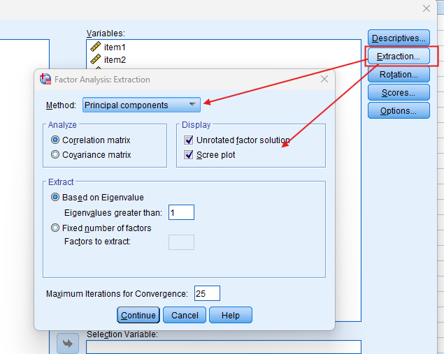
4. Choose Extraction Method:

– Click on the `Extraction` button and select an extraction method such as Principal Component Analysis (PCA) or Principal Axis Factoring (PAF). Ensure you choose the number of factors to extract or use the default criteria.

5. Apply Rotation:

– Click on the `Rotation` button and choose a rotation method (e.g., Varimax, Direct Oblimin) to enhance the interpretability of the factor structure.

6. Run the Analysis:

– Click OK to run the analysis. SPSS will generate output tables detailing the factor loadings, eigenvalues, and explained variance.

By following these steps, you can effectively perform an Exploratory Factor Analysis in SPSS, ensuring accurate and interpretable results.

Note: Conducting EFA in SPSS provides a robust foundation for understanding the key features of your data. Always ensure that you consult the documentation corresponding to your SPSS version, as steps might slightly differ based on the software version in use. This guide is tailored for SPSS version 25, and for any variations, it’s recommended to refer to the software’s documentation for accurate and updated instructions.

How to Interpret SPSS Output of Factor Analysis

KMO and Bartlett’s Test

Firstly, the KMO value indicates the suitability of your data for factor analysis. Values closer to 1 suggest that your data is highly factorable, making it ideal for exploratory factor analysis in SPSS. Moreover, Bartlett’s Test of Sphericity checks if your correlation matrix is significantly different from an identity matrix. If this test is significant, it indicates that factor analysis is appropriate for your data.

Correlation Matrix

The Correlation Matrix displays Pearson correlation coefficients between pairs of items. High correlations suggest that the items may share underlying factors, which is crucial for exploratory factor analysis in SPSS. Furthermore, it helps identify multicollinearity and determine the suitability of items for factor analysis. This ensures that the items are appropriate for uncovering latent constructs.

Communalities

Communalities represent the proportion of each variable’s variance that the factors can explain. Higher communalities indicate that a large portion of the variable’s variance is accounted for by the extracted factors, which is essential for reliable factor analysis. Initially, communalities show the variance accounted for by the initial solution. Subsequently, extraction communalities show the variance accounted for by the retained factors, providing a clear picture of the factors’ effectiveness.

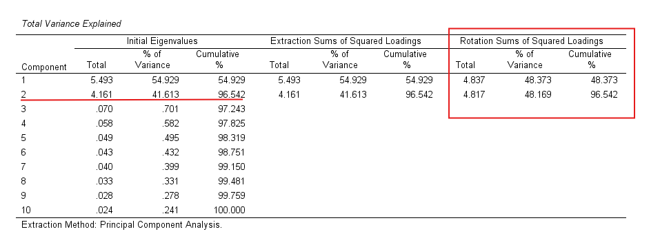
Total Variance Explained

This table provides eigenvalues and the percentage of variance explained by each factor, which is vital for determining factor significance. Factors with eigenvalues greater than 1 are typically retained, ensuring that only meaningful factors are considered. Additionally, the table shows the cumulative percentage, indicating how much of the total variance is explained by the extracted factors. This helps in understanding the overall impact of the factors on the dataset.

Scree Plot

The Scree Plot is a graphical representation of the eigenvalues associated with each factor. It helps determine the number of factors to retain by identifying the “elbow point,” where the eigenvalues start to level off. Factors above this point are typically retained, while those below are considered less significant. This method ensures a clear and straightforward factor solution for your analysis.

Component Matrix

The Component Matrix shows the factor loadings of each variable before rotation. Factor loadings indicate the correlation between the variable and the factor. Loadings closer to 1 or -1 indicate a strong relationship, while loadings closer to 0 indicate a weak relationship.

Rotated Component Matrix

The Rotated Component Matrix displays the factor loadings after rotation, making the factor structure easier to interpret. Rotation maximises the loadings of variables on a single factor and minimises loadings on other factors. Common rotation methods include Varimax, Direct Oblimin, and Promax.

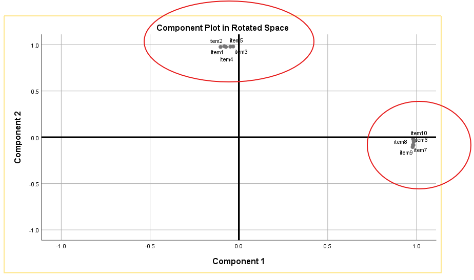
Component Plot of Factors

The Component Plot visually represents the factors in a two-dimensional space, showing the relationships among the variables. This plot helps in understanding the clustering of variables and their association with the factors. It provides a visual confirmation of the factor structure identified in the analysis.

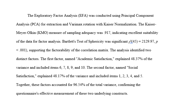
How to Report Results of Factor Analysis in APA

• Introduction: Briefly describe the purpose of the EFA and the variables included in the analysis.
• Factor Extraction: Describe the extraction method used (e.g., PCA, PAF) and the criteria for determining the number of factors (e.g., eigenvalues greater than 1, Scree Plot).
• Rotation Method: Specify the rotation method applied (e.g., Varimax, Direct Oblimin) and explain why it was chosen.
• Factor Loadings: Provide the factor loadings for each variable, indicating which items load onto which factors.
• Variance Explained: Report the percentage of variance explained by each factor and the cumulative variance.
• Interpretation: Discuss the meaning of the factors and the variables that load onto each factor, providing insights into the underlying constructs.
• Figures and Tables: Include tables and figures to visually represent the factor loadings, Scree Plot, and other relevant statistics.
• Conclusion: Summarise the key findings, implications for theory and practice, and suggest directions for future research.

By following these guidelines, you can effectively report the results of your Exploratory Factor Analysis in accordance with APA standards, ensuring clarity and comprehensibility for your audience.

Get Help For Your SPSS Analysis

Embark on a seamless research journey with SPSSAnalysis.com, where our dedicated team provides expert data analysis assistance for students, academicians, and individuals. We ensure your research is elevated with precision. Explore our pages;

• SPSS Help by Subjects Area: Psychology, Sociology, Nursing, Education, Medical, Healthcare, Epidemiology, Marketing 
• Dissertation Methodology Help
• Dissertation Data Analysis Help
• Dissertation Results Help
• Pay Someone to Do My Data Analysis
• Hire a Statistician for Dissertation
• Statistics Help for DNP Dissertation
• Pay Someone to Do My Dissertation Statistics

Connect with us at SPSSAnalysis.com to empower your research endeavors and achieve impactful data analysis results. Get a FREE Quote Today!