Normality Test in SPSS
Discover the Normality Test in SPSS! Learn how to perform, understand SPSS output, and report results in APA style. Check out this simple, easy-to-follow guide below for a quick read!
Struggling with the Normality test in SPSS? We’re here to help. We offer comprehensive assistance to students, covering assignments, dissertations, research, and more. Request Quote Now!

Introduction
In the realm of statistical analysis, ensuring the data conforms to a normal distribution is pivotal. Researchers often turn to Normality Tests in SPSS to evaluate the distribution of their data. As statistical significance relies on certain assumptions, assessing normality becomes a crucial step in the analytical process. This blog post delves into the intricacies of Normality Tests, shedding light on tools like the Kolmogorov-Smirnov test and Shapiro-Wilk test, and exploring the steps involved in examining normal distribution using SPSS.
Normal Distribution Test
A Normal Distribution Test, as the name implies, is a statistical method employed to determine if a dataset follows a normal distribution. The assumption of normality is fundamental in various statistical analyses, such as t-tests and ANOVA. In the context of SPSS, researchers utilize tests like the Kolmogorov-Smirnov test and Shapiro-Wilk test to ascertain whether their data conforms to the bell-shaped curve characteristic of a normal distribution. This initial step is crucial as it influences the choice of subsequent statistical tests, ensuring the robustness and reliability of the analytical process. Moving forward, we will dissect the significance and objectives of conducting Normality Tests in SPSS.
Aim of Normality Test
Exploring the data is a fundamental step in statistical analysis, and SPSS offers a comprehensive tool called Explore Analysis for this purpose.
The Analysis provides a detailed overview of the dataset,
- presenting essential descriptive statistics,
- measures of central tendency, and
- dispersion
The primary aim of a Normality Test is to evaluate whether a dataset adheres to the assumptions of a normal distribution. This is pivotal because many statistical analyses, including parametric tests, assume that the data is normally distributed.
Assumption of Normality Test
Understanding the assumptions underpinning the Normality Test is crucial for accurate interpretation. Firstly, it’s essential to acknowledge that many parametric tests assume a normal distribution of data for valid results. Consequently, the assumption of normality ensures that the sampling distribution of a statistic is approximately normal, which, in turn, facilitates the application of inferential statistics. Therefore, by subjecting the data to a Normality Test, researchers validate this assumption, providing a solid foundation for subsequent analyses.
How to Check Normal Distribution in SPSS
To comprehensively check for normal distribution in SPSS, researchers can employ a multifaceted approach. Firstly, visual inspection through a Histogram can reveal the shape of the distribution, offering a quick overview. The Normal Q-Q plot provides a graphical representation of how closely the data follows a normal distribution. Additionally, assessing skewness and kurtosis values adds a numerical dimension to the evaluation. High skewness and kurtosis values can indicate departures from normality. Lastly, we can check with statistical tests such as the Kolmogorov-Smirnov test, and the Shapiro-Wilk test. This section will guide users through the practical steps of executing these checks within the SPSS interface, ensuring a thorough examination of the dataset’s distributional characteristics.
1. Kolmogorov-Smirnov Test
The Kolmogorov-Smirnov test, often abbreviated as the K-S test, is a non-parametric method for determining whether a sample follows a specific distribution. In the context of SPSS, this test is a powerful tool for assessing the normality of a dataset. By comparing the empirical distribution function of the sample with the expected cumulative distribution function of a normal distribution, the K-S test quantifies the degree of similarity.
2. Shapiro-Wilk Test
An alternative to the Kolmogorov-Smirnov test, the Shapiro-Wilk test is another statistical method used to assess the normality of a dataset. Particularly effective for smaller sample sizes, the Shapiro-Wilk test evaluates the null hypothesis that a sample is drawn from a normal distribution. SPSS facilitates the application of this test, offering a straightforward process for researchers.
4. Histogram Plot
Utilizing a Histogram Plot in SPSS is a visual and intuitive method for determining normal distribution. By representing the distribution of data in a graphical format, researchers can promptly identify patterns and deviations.
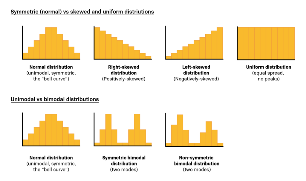
Here are some common shapes of histograms and their explanations:
- Normal Distribution (Bell Curve): It has a symmetrical, bell-shaped curve. The data is evenly distributed around the mean, forming a characteristic bell curve. The majority of observations cluster around the mean, with fewer observations towards the tails.
- Positively Skewed (Skewed Right): The right tail is longer than the left. Most of the data is concentrated on the left side, and a few extreme values pull the mean to the right. This shape is often seen in datasets with a floor effect, where values cannot go below a certain point.
- Negatively Skewed (Skewed Left): It has a longer left tail. The majority of data points are concentrated on the right side, with a few extreme values dragging the mean to the left. This shape is common in datasets with a ceiling effect, where values cannot exceed a certain point.
Other Distributions
- Bimodal: It has two distinct peaks, indicating the presence of two separate modes or patterns in the data. This shape suggests that the dataset is a combination of two different underlying distributions.
- Uniform: All values have roughly the same frequency, resulting in a flat, rectangular shape. There are no clear peaks or valleys, and each value has an equal chance of occurrence.
- Multimodal: It has more than two peaks, indicating multiple modes in the dataset. Each peak represents a distinct pattern or subgroup within the data.
- Exponential: It has a rapidly decreasing frequency as values increase. It is characterized by a steep decline in the right tail. The shape is common in datasets where the likelihood of an event decreases exponentially with time.
- Comb: It has alternating high and low frequencies, creating a pattern that resembles the teeth of a comb. This shape suggests periodicity or systematic variation in the data.
5. Normal Q-Q Plot
Furthermore, the Normal Q-Q plot complements the Histogram by providing a visual comparison between the observed data quantiles and the quantiles expected in a normal distribution. By comparing observed quantiles with expected quantiles, researchers gain insights into the conformity of the data to a normal distribution. Clear instructions ensure a seamless incorporation of this method into the normality checking process.
6. Skewness and Kurtosis
Skewness
It is a statistical measure that quantifies the asymmetry of a probability distribution or a dataset. In the context of data analysis, skewness helps us understand the distribution of values in a dataset and whether it is symmetric or not. The value can be positive, negative, or zero.
- Positive: it indicates that the data distribution is skewed to the right. In other words, the tail on the right side of the distribution is longer or fatter than the left side, and the majority of the data points are concentrated towards the left.
- Negative: Conversely, the data distribution is skewed to the left. The tail on the left side is longer or fatter than the right side, and the majority of data points are concentrated towards the right.
- Zero: A skewness value of zero suggests that the distribution is perfectly symmetrical, with equal tails on both sides.
In summary, skewness provides insights into the shape of the distribution and the relative concentration of data points on either side of the mean.
Kurtosis
It is a statistical measure that describes the distribution’s “tailedness” or the sharpness of the peak of a dataset. This helps to identify whether the tails of a distribution contain extreme values. Like skewness, kurtosis can be positive, negative, or zero.
- Positive: The distribution has heavier tails and a sharper peak than the normal distribution. So, It suggests that the dataset has more outliers or extreme values than would be expected in a normal distribution.
- Negative: Conversely, the distribution has lighter tails and a flatter peak than the normal distribution. Therefore, It implies that the dataset has fewer outliers or extreme values than a normal distribution.
- Zero: A kurtosis value of zero, also known as mesokurtic, indicates a distribution with tails and a peak similar to the normal distribution.
In data analysis, For a normal distribution, skewness is close to zero, and kurtosis is around 3 (known as mesokurtic). Deviations from these values may suggest non-normality and guide researchers in choosing appropriate statistical methods.
Example of Normality Test
To provide practical insights, this section will present a hypothetical example illustrating the application of normality tests in SPSS. Through a step-by-step walkthrough, readers will gain a tangible understanding of how to apply the Kolmogorov-Smirnov and Shapiro-Wilk tests to a real-world dataset, reinforcing the theoretical concepts discussed earlier.
Scenario:
Imagine you are a researcher conducting a study on the screen time of a group of individuals. You have collected data on the number of min each participant’s screen time per day. As part of your analysis, you want to assess whether the phone screen time follows a normal distribution. Let’s see how to conduct explore analysis in SPSS.


Step by Step: Running Normality Analysis in SPSS Statistics
Practicality is paramount, and this section will guide researchers through the step-by-step process of performing a Normality Test in SPSS. From importing the dataset to interpreting the results, this comprehensive guide ensures seamless execution of the normality testing procedure, fostering confidence in the analytical journey.
- STEP: Load Data into SPSS
Commence by launching SPSS and loading your dataset, which should encompass the variables of interest – a categorical independent variable. If your data is not already in SPSS format, you can import it by navigating to File > Open > Data and selecting your data file.
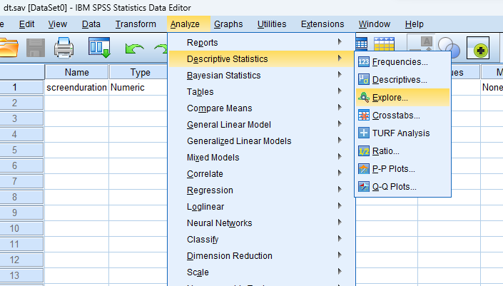
- STEP: Access the Analyze Menu
In the top menu, locate and click on “Analyze.” Within the “Analyze” menu, navigate to “Descriptive Statistics” and choose ” Explore.” Analyze > Descriptive Statistics > Explore
- STEP: Specify Variables
Upon selecting “ Explore ” a dialog box will appear. Choose the variable of interest and move it to the “Dependent List” box
- STEP: Define Statistics
Click on the ‘Statistics’ button to include Descriptives, Outliers, and Percentiles.
- STEP: Define the Normality Plot with the Test
Click on the ‘Plot’ button to include visual representations, such as histogram, and stem-and-leaf. Check “Normality plots with tests” to obtain a Normal Q-Q plot, Kolmogorov-Smirnov Test, and Shapiro-Wilk test.
6. Final STEP: Generate Normality Test and Chart:
Once you have specified your variables and chosen options, click the “OK” button to perform the analysis. SPSS will generate a comprehensive output, including the requested frequency table and chart for your dataset.
Note:
Conducting the Normality Test in SPSS provides a robust foundation for understanding the key features of your data. Always ensure that you consult the documentation corresponding to your SPSS version, as steps might slightly differ based on the software version in use. This guide is tailored for SPSS version 25, and any variations, it’s recommended to refer to the software’s documentation for accurate and updated instructions.


How to Interpret SPSS Output of Normality Test
Interpreting the output of a normality test is a critical skill for researchers. This section will dissect the SPSS output, explaining how to analyze results from the Kolmogorov-Smirnov and Shapiro-Wilk tests, as well as interpret visual aids like Histograms and Normal Q-Q plots.
- Skewness and Kurtosis: The skewness of approximately 0 suggests a symmetrical distribution, while the negative kurtosis of -0.293 indicates lighter tails compared to a normal distribution.
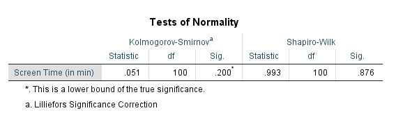
- Kolmogorov-Smirnov Test: The Kolmogorov-Smirnov test yields a statistic of 0.051 with a p-value of 0.200 (approximately), indicating no significant evidence to reject the null hypothesis of normality.
- Shapiro-Wilk Test: The Shapiro-Wilk test produces a statistic of 0.993 with a p-value of 0.876, providing further support for the assumption of normality.
- Histogram and Normal Q-Q Plot: The Histogram with a central peak, reflects a symmetric distribution, and the Normal Q-Q plot with points closely aligned along a straight line, affirming the approximate normality of the “Screen Time (in min)” variable.
How to Report Results of Normality Analysis in APA
Effective communication of research findings is essential, and this section will guide researchers on how to report the results of normality tests following the guidelines of the American Psychological Association (APA). From structuring sentences to incorporating statistical values, this segment ensures that researchers convey their findings accurately and professionally.

Get Help From SPSSanalysis.com
Embark on a seamless research journey with SPSSAnalysis.com, where our dedicated team provides expert data analysis assistance for students, academicians, and individuals. We ensure your research is elevated with precision. Explore our pages;
- SPSS Data Analysis Help – SPSS Helper,
- Quantitative Analysis Help,
- Qualitative Analysis Help,
- SPSS Dissertation Analysis Help,
- Dissertation Statistics Help,
- Statistical Analysis Help,
- Medical Data Analysis Help.
Connect with us at SPSSAnalysis.com to empower your research endeavors and achieve impactful results. Get a Free Quote Today!