Meta Analysis for Continuous Outcome in SPSS
Discover Meta Analysis for Continuous Outcome in SPSS! Learn how to perform, understand SPSS output, and report results in APA style. Check out this simple, easy-to-follow guide below for a quick read!
Struggling with Meta Analysis in SPSS? We’re here to help. We’re here to help. We provide comprehensive support to academics and PhD students, encompassing assignments, dissertations, research, and additional services. Request Quote Now!

1. Introduction
Meta-analysis for continuous outcomes is a widely used method for synthesizing mean differences across multiple studies. It is essential in clinical research, psychology, and education when outcomes are measured on numeric scales. SPSS offers tools and macros to conduct such analyses efficiently, including effect size calculations and model estimations.
This blog post introduces you to Meta-Analysis with Continuous Outcome in SPSS, explains its methods, and walks through a detailed example to help you perform and interpret this analysis effectively.
2. What is Meta-Analysis for Continuous Outcomes?
This type of meta-analysis combines effect sizes from studies reporting continuous variables, such as blood pressure, depression scores, or cognitive performance. The analysis accounts for variation across studies and produces a pooled estimate of the mean difference or standardized effect size.
In addition to continuous outcomes, meta-analysis can be applied to other data types depending on the study design and reported results. Common types include:
- Binary Outcome Meta-Analysis: Binary meta-analysis refers to the statistical synthesis of results from studies with dichotomous outcomes, such as event/no-event, success/failure, or improved/not improved.
- Meta-Regression: Meta-regression examines whether study-level variables (e.g., sample size, year, dosage) explain variation in effect sizes. It’s ideal when heterogeneity is present.
- Proportional Meta-Analysis: Used to pool proportions or prevalence data (e.g., infection rates). Logit transformation is often applied to stabilize variance. This method is common in epidemiology and can be implemented in SPSS .
3. When to Use Continuous Meta Analysis?
Continuous meta-analysis is used when the outcome variable in each study is measured on a continuous scale—such as blood pressure, anxiety scores, weight, or test performance. These outcomes are reported as means and standard deviations, allowing researchers to compare differences across groups or time points.
You should use continuous meta-analysis when:
-
Studies report means and standard deviations for treatment and control groups.
-
Outcomes are numeric and measured on interval or ratio scales, not categorical or binary.
-
You want to calculate standardized effect sizes (e.g., Cohen’s d or Hedges’ g) to compare results across studies that may use different scales.
-
Your goal is to estimate the overall treatment effect, accounting for sampling variability and potential between-study differences.
SPSS V28+ allows continuous meta-analysis using both raw data (means, SDs, n) and pre-calculated effect sizes. This makes it ideal for synthesizing evidence when evaluating continuous treatment effects.
4. What Effect Size for Continuous Outcome in Meta Analysis?
In SPSS, you can choose from several effect sizes for continuous outcome meta-analysis. Here’s a breakdown with guidance:
-
Cohen’s d: Standardized mean difference using pooled standard deviation.
-
Hedges’ g: Adjusted version of Cohen’s d, recommended for small samples.
-
Glass’s Δ: Uses only the control group’s standard deviation, suitable when variability differs across groups.
-
Unstandardized Mean Difference (UMD): Used when all studies measure outcomes on the same scale.
Best Practice: Use UMD when units are consistent. Use Hedges’ g when standardization is needed, especially for small sample studies.
5. What is the Difference Between Fixed and Random effects?.
-
Fixed-effect model assumes all studies estimate the same true effect.
-
Random-effects model allows for study-to-study variability, assuming true effects vary around a mean.
Best Option: Use random-effects when heterogeneity is expected, which is common in real-world data.
6. What Estimator Type of Meta Analysis of Continuous Outcome?
SPSS allows choosing from several estimators to calculate the pooled effect under a random-effects model:
-
REML (Restricted Maximum Likelihood): Offers stable and unbiased estimates; widely preferred.
-
ML (Maximum Likelihood): Can underestimate variance; less ideal for small samples.
-
Empirical Bayes: Shrinks extreme estimates toward the mean; useful with prior distributions.
-
Hunter-Schmidt: Corrects for measurement error; used in psychometric contexts.
-
Hedges: Adjusts for small sample bias.
-
DerSimonian-Laird: Common default, though may overestimate precision.
-
Sidik-Jonkman: More robust under high heterogeneity.
Best Choice: For most continuous outcome meta-analyses, use REML for more stable estimates of heterogeneity and pooled effects.
7. Which Standard Error Adjustment Should You Set?
SPSS allows adjusting the standard error (SE) of the pooled estimate to correct for small sample bias:
-
No Adjustment: Assumes normality and homogeneity; less conservative.
-
Knapp-Hartung (KH): Provides more conservative standard errors; better with few studies.
-
Truncated Knapp-Hartung: A modified version to avoid excessively wide CIs.
Best Practice: Knapp-Hartung is advised when dealing with fewer than 10 studies or high heterogeneity.
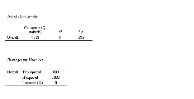
8. Heterogeneity in Meta Analysis of Continuous Outcome
Heterogeneity assesses variation among study results and is quantified using:
-
Q-statistic: Tests for heterogeneity. (with df and p-value)
-
I² statistic: Proportion of variability due to heterogeneity (≥ 50% indicates moderate-to-high).
-
Tau²: Variance of true effect sizes.
Exploring sources of heterogeneity is essential before drawing firm conclusions.
9. What is Trim and Fill in Meta Analysis?
Trim and Fill is a statistical method used to detect and adjust for publication bias in meta-analyses, including those with continuous outcomes. It starts by assessing asymmetry in the funnel plot, which may indicate that smaller studies with non-significant results are missing from the published literature.
The method “trims” the asymmetric studies and estimates how many studies are likely missing. It then “fills” in these hypothetical studies to create a more symmetrical funnel plot and recalculates the pooled effect size accordingly.
Although Trim and Fill does not remove publication bias, it offers a sensitivity analysis. This helps researchers evaluate whether the overall findings are robust in the presence of possible missing or unpublished studies.
10. How Subgroup Analysis Works
Subgroup analysis explores whether the treatment effect varies across different categories of studies. For continuous outcomes, studies can be grouped based on categorical moderators such as:
-
Type of intervention
-
Geographic region
-
Study quality
-
Population characteristics (e.g., age group, clinical setting)
In SPSS, subgroup analysis is typically performed using a mixed-effects model. This approach estimates separate pooled effect sizes for each subgroup and compares them to assess whether the moderator variable explains heterogeneity. If between-group differences are statistically significant, it suggests that the moderator may influence the effect size.
Subgroup analysis is especially useful when heterogeneity is present and helps generate hypotheses for future research.
11. What is Publication Bias in Meta Analysis of Continuous Outcome?
Publication bias occurs when studies with null or negative results remain unpublished. Common tests include:
-
Egger’s Test: Assesses asymmetry in the funnel plot.
-
Peters’ Test: Alternative method more suitable for binary outcomes but sometimes referenced.
-
Harbord Test: Similar to Egger’s but designed for odds ratios.
Each test has its assumptions; use more than one when possible.
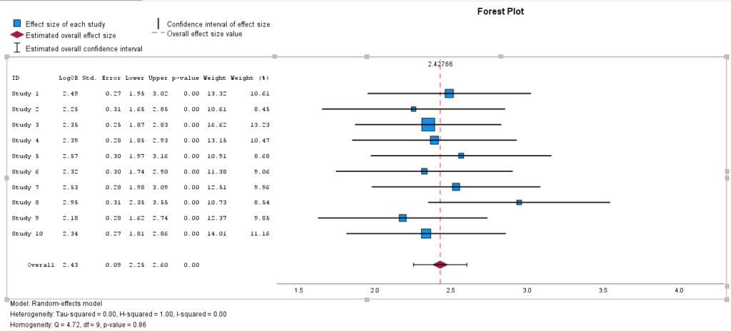
12. What is Used for a Funnel and Forest Plot in Meta Analysis?
-
Forest Plot: Summarises effect sizes and confidence intervals visually across studies.
-
Funnel Plot: Detects potential publication bias based on the symmetry of effect sizes.
SPSS generates both plots automatically in continuous meta-analysis using the appropriate chart options.
13. What Are the Assumptions of Meta-Analysis for Continuous Outcome?
-
Independent effect sizes across studies
-
Normally distributed sampling errors
-
Consistent measurement or appropriately standardized outcomes
-
Homogeneity or accounted-for heterogeneity via random-effects model
14. An Example for Meta Analysis for Continuous Outcome
Suppose 12 trials assess the effect of a cognitive training intervention on memory scores. Each reports mean, SD, and sample size per group. After calculating Cohen’s d for each study, a random-effects meta-analysis is conducted. Results show a moderate pooled effect size with low heterogeneity and no evidence of publication bias.

In the following sections, we’ll explain how to perform such an analysis in SPSS. For this example, we will use SPSS v.30, but you can use Meta MACRO from the original meta-analysis utilities by Prof. David Wilson.
15. How to Perform Meta Analysis for Continuous in SPSS


Step by Step: Running Continuous Meta-Analysis in SPSS Statistics
Let’s embark on a step-by-step guide on performing the continuous meta-analysis using SPSS
In SPSS version 28 and higher, you can directly conduct meta-analysis for Continuous outcomes using the native interface. The procedure supports two approaches:
-
Enter raw data (means, SDs, sample sizes)
-
Enter pre-calculated effect sizes (e.g., Cohen’s d and standard error already calculated)
To perform continuous meta-analysis in SPSS:
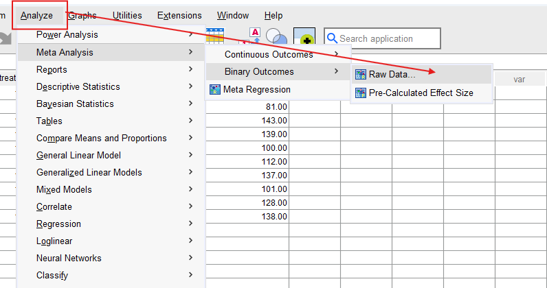
1. STEP: Go to Analyze → Meta Analysis → Continuous Outcome.
2. STEP: Choose the appropriate input:
- If you have raw data (e.g., means, SDs and sample sizes), select Effect sizes not available.
- If you have already computed Cohen’s d or Hedges’ g and SE, select Effect sizes available.
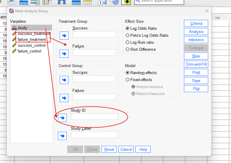
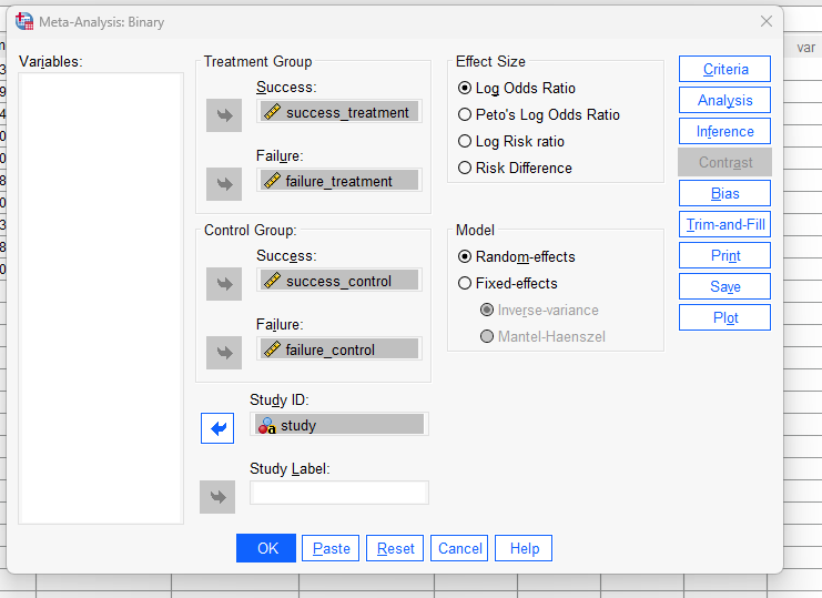
3. STEP: In the Variables tab:
- For raw data, assign: means, SDs, and sample sizes for the treatment and control groups.
- For calculated data, assign: Effect size variable (e.g., Cohen’s d or Hedges’ g) and Standard error or variance.
4. STEP: In the Inference tab:
- Choose between Fixed effects or Random effects.
- Select the estimator (e.g., REML, DL, Sidik-Jonkman).
- Set standard error adjustment (e.g., Knapp-Hartung).
5. STEP: Optionally, explore:
- Bias, Trim-and-Fill tabs for subgroup or meta-regression analyses.
- Plots tab to produce forest and funnel plots.
6. STEP: Click OK to run the analysis.
SPSS will produce output with pooled estimates, heterogeneity statistics, and visualizations.
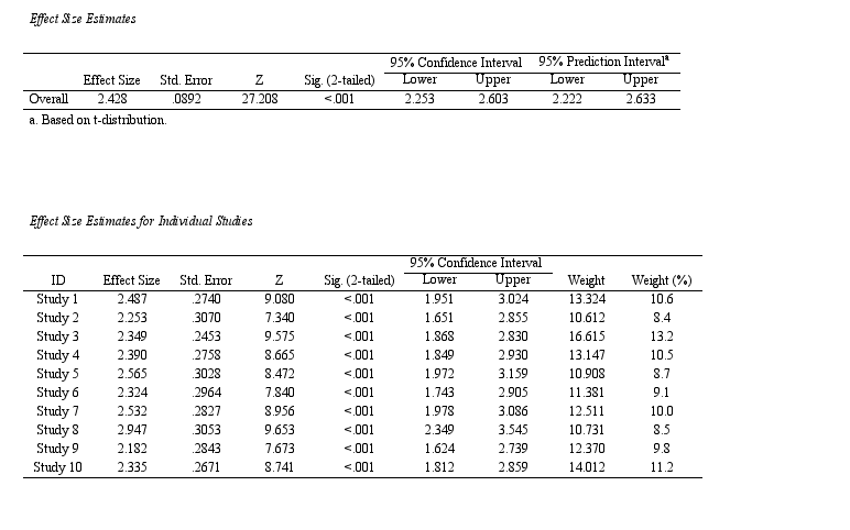
SPSS Output for Continuous Meta Analysis

17. How to Interpret SPSS Output of Continuous Meta Analysis
Once the analysis is complete, SPSS generates a detailed output including pooled effect estimates, confidence intervals, heterogeneity indices, and plots.
Key components to interpret:
-
Pooled Effect Size: Represents the overall estimate. A significant effect (e.g., Hedges’ g = 0.45, 95% CI [0.30, 0.60]) indicates a meaningful association across studies.
-
Heterogeneity Statistics:
-
Q-test: Tests whether effect sizes are more variable than expected by chance. A significant result suggests heterogeneity.
-
I²: Describes the percentage of total variation due to heterogeneity. Interpret as:
-
0–40%: low
-
30–60%: moderate
-
50–90%: substantial
-
75–100%: considerable
-
-
Tau²: The estimated between-study variance. A larger τ² indicates more between-study variability.
-
-
Forest Plot: Displays effect size and confidence intervals for each study and the pooled estimate.
-
Funnel Plot (optional): Used to assess publication bias. Asymmetry may indicate bias or small-study effects.
-
Moderator Analyses: If subgroup variables are included, SPSS will display pooled estimates per group, and test for differences between them.
18. How to Report Results of Meta Analysis in APA
- Study Selection Summary: Report the total number of studies identified, screened, and included in the meta-analysis. Indicate any exclusions and provide a brief narrative consistent with the PRISMA flow diagram.
- Study Characteristics: Summarize key characteristics of the included studies, such as study design, sample sizes, outcome definitions, and population types. Mention whether studies used similar methods or settings.
- Effect Size and Model: Specify the effect size metric used (e.g., Cohen’s d, Hedges’ g ). Indicate whether a fixed-effect or random-effects model was applied, and name the estimator (e.g., REML, ML, DL).
- Heterogeneity: Report heterogeneity statistics including the Q statistic with degrees of freedom and p-value. Also include I² (%) to quantify inconsistency and τ² to reflect between-study variance.
- Publication Bias: Describe whether publication bias was assessed. Mention the use of funnel plots and any statistical tests (e.g., Egger’s, Harbord, Peters). Indicate whether the trim-and-fill method was applied and if it affected the pooled estimate.
- Subgroup and Sensitivity Analyses: If applicable, describe subgroup analyses performed based on categorical moderators (e.g., region, study quality). Report sensitivity analyses used to assess robustness of results (e.g., leave-one-out analysis, exclusion of outliers).
- Pooled Results Summary: Present the pooled effect size with its 95% confidence interval and p-value. Interpret the direction, magnitude, and statistical significance of the effect in context. Optionally, include the 95% prediction interval if available.

Get Help For Your SPSS Analysis
Embark on a seamless research journey with SPSSAnalysis.com, where our dedicated team provides expert data analysis assistance for students, academicians, and individuals. We ensure your research is elevated with precision. Explore our pages;
- Meta Analysis in Clinical Research
- Meta Analysis in Psychology
- Dissertation Help Statistics
- Dissertation Analysis Help
- Online Statistics Help
- SPSS Help by Subject Area: Psychology, Sociology, Nursing, Education, Medical, Healthcare, Epidemiology, Marketing
Connect with us at SPSSAnalysis.com to empower your research endeavors and achieve impactful data analysis results. Get a FREE Quote Today!
PS: This guide is tailored for SPSS version 30, and for any variations, it’s recommended to refer to the software’s documentation for accurate and updated instructions.